| Issue |
Emergent Scientist
Volume 5, 2021
|
|
|---|---|---|
| Article Number | 3 | |
| Number of page(s) | 9 | |
| Section | Physics | |
| DOI | https://doi.org/10.1051/emsci/2021002 | |
| Published online | 20 May 2021 | |
Research Article
The Gauss pendulum
Center for Engineering, Modeling and Applied Social Sciences of the Federal University of ABC. Av. dos Estados,
5001 - Bangú, Santo André – SP,
09210-580,
Santo André,
Brazil
* e-mail: This email address is being protected from spambots. You need JavaScript enabled to view it.
Received:
7
September
2020
Accepted:
8
March
2021
Abstract
Recently, the Gauss rifle has gained attention as an interesting problem for physics and engineering education. In this manuscript we propose and analyze a novel problem that, while being related to the Gauss rifle, is rather simpler: the Gauss pendulum, which yields more consistent results and allows further agreement between model, simulation and experimental data. The Gauss pendulum, unlike the rifle, does not involve rotational movement of balls and the difference between the initial and final energy state of the system can be easily accessed by measuring the final height of the swinging projected ball. An extensive assessment of a Gauss pendulum has been developed using free software and accessible laboratory equipment. Focusing on the validation of the magnetic potential well model to understand the gain in kinetic energy, it was possible to obtain a remarkable agreement between the experimental and theoretically simulated data.
Key words: Gauss rifle / Newton’s cradle / physics experiment / magnetic materials / magnetism / pendulum.
© J. C. Teixeira et al., published by EDP Sciences, 2021
 This is an Open Access article distributed under the terms of the Creative Commons Attribution License (https://creativecommons.org/licenses/by/4.0), which permits unrestricted use, distribution, and reproduction in any medium, provided the original work is properly cited.
1 Introduction
Accelerating projectiles using magnetic fields instead of gun powder or other chemical propellants have been studied since the 19th century. Recently, the US Navy revealed a weapon in advanced stage of development, the railgun, which is based on this principle [1]. While chemical propellant weapons can accelerate projectiles up to 2 km/s muzzle velocities, railguns can reach up to 3 km/s.
More recently, a device using a different method to magnetically accelerate a projectile has drawn attention from the university community and amateur developers. This device is known as the Gauss rifle (the terms “gun” and “cannon” are also used) and employs strong magnets and steel balls [2]. To those who are not familiar with the Gauss rifle we suggest to take a few minutes to watch the educational video made by our group, available on the internet [3]. The Gauss rifle has been considered an interesting problem for physics and engineering projects [4–7].
In this manuscript we put forward the concept of the Gauss pendulum, a new setup devoted to the study of magnetically accelerated projectiles. Its principle of operation is akin to the Gauss rifle and offers advantages and new learning possibilities.
Firstly, we will discuss the similarities and differences of the Gauss rifle and Gauss pendulum, in order to allow further analysis on the latter.
1.1 The Gauss rifle
A sketch of a Gauss gun is depicted in Figure 1. It consists of a magnet associated with steel balls resting on a rail. For practical reasons, the magnet is fixed on the rail, but this is not truly necessary. The balls are made of ferromagnetic steel and are usually taken from ball bearings. The magnetic character of the projectile is of fundamental relevance for the workings of the rifle. The role of the rail is to reduce the freedom of movement of the spheres into one dimension with the least possible friction. The figure shows the setup using three balls, which is the minimum amount of balls necessary for the gun to work. This setup is assembled in such a way that two balls are magnetically attached to one side of the magnet: the ball which is further away from the magnet works as the projectile and the second one works as a spacer. More balls can be used as spacers. The third ball is used as a trigger. In this figure, the Gauss rifle depicted has only one stage, (assembly with balls and a magnet), but it is possible to build rifles with several stages.
The process of the Gauss rifle shot is usually described by four different steps:
-
A trigger ball is rolled towards the magnet.
-
The trigger ball gains kinetic energy due to the magnetic attraction and collides with the magnet.
-
In a way akin to Newton’s cradle, the kinetic energy is transferred from the trigger ball to the projectile ball.
-
The projectile moves away from the magnet and its final velocity is higher than the initial velocity of the trigger ball.
Although it is gaining popularity as a learning tool for physicists and engineers, we can list three main disadvantages of the Gauss rifle assembly, which make the question of energy conservation hard to assess:
-
It is difficult to calculate what are the rotational and translational contributions to the total kinetic energy of the balls (trigger and projectile). In an ideal situation, the balls should roll without friction on the rail. As for the trigger ball, the magnetic force in the last couple of millimeters of the approximation to the magnet is orders of magnitude higher than the static friction force which makes the trigger ball roll without slipping on the rail [6,8]. As a result, in the last millimeters, this ball is accelerated so strongly that it slips towards the magnet. The opposite happens with the projectile: the impulse it gets from the assembly is essentially linear and rather strong, therefore the kinetic energy of the projectile is initially linear. The rotational energy gradually comes into play as the friction force against the rail prompts the ball to roll.
-
The kinetic energy gained by the trigger ball due to the magnetic force is transferred to the projectile ball by a Nesterenko soliton [2] propagating through the elements of the assembly in a similar way that happens in a Newton’s cradle [9]. However, in the latter, the elements of the chain are identical and, in a first approximation, all kinetic energy from the trigger ball is transferred to the projectile. This is not the case for the Gauss rifle, where the magnet is present along with the balls and the assembly is no longer homogeneous. As a result, part of the energy of the soliton is not transferred but rather reflected, generating recoil. As already mentioned, the magnet is fixed to the rail for practical reasons and the recoil energy is dissipated and hardly assessed. There is yet another relevant difference between the collision mechanics featured by the Newton’s Cradle and the Gauss rifle: in the latter case, the trigger ball, although slipping in the last moment, still retains a good portion of rotational energy from the approximation process; in the former case, the movement of the balls is essentially linear.
-
Modelling, simulating and assessing the magnetic interactions of the magnet and ball bearings can be rather tricky [2,6]. Part of the problem is related to the rotation of the balls, which are made of ferromagnetic steel, although they are not permanent magnets. As a result, their magnetization tends to align to the external magnetic field generated by the overall interaction between the magnet and the ball bearings in the assembly. The rotation of the steel balls adds another layer of complication and other sources of energy loss due to the continuous magnetization realignment and hysteresis.
It is worth noting that, although the above mentioned aspects are relevant, they can be circumvented with moderate success using a few ad hoc assumptions [2] [6].
1.2 The Gauss pendulum
In this context, we put forward the idea of a simpler setup that we call the Gauss pendulum, in which we combine the physical phenomena of the Gauss rifle with the Newton’s cradle. It should be recalled that the Newton’s cradle has also been used for similar projects [10]. In Figure 2, it is possible to see two main advantages with the Gauss pendulum: it avoids the three complications listed above; and it allows the assessment of its efficiency by evaluating its final energy. This is done by another simple and reliable energy conservation process: from kinetic energy to gravitational potential energy. In this way, the recoil effect can be measured and the energy losses are mostly related to the coefficient of restitution inherent of the Nesterenko soliton process.
It is possible to model this transformation of magnetic energy into kinetic energy using the concept of a potential well. This analogy can be used in order to understand energy conservation both in the Gauss rifle and in the Gauss pendulum. If we leave aside the rotational aspect of the balls, this simple model explains both devices accordingly. In Figure 3 we sketched a mixed metaphor diagram representing the initial and final stages of the interaction, in order for it to be correlated with the initial and final stages of Figures 1 and 2. The term “mixed metaphor” is used here because, although this analogy can be useful to comprehend the phenomenon, one has to be careful not to over-interpret the sketch. This pictorial representation of the energy transformation process of the Gauss rifle has been put forward by our group previously [3] and a 3D printed analog has been presented by another group later on [11].
In the moment a Gauss rifle or pendulum experiment is performed, the most striking fact observed is the increase in kinetic energy of the projectile when compared to the trigger ball. In order to aid the understanding of this aspect, Figure 3 illustrates the initial and final states of the process. The vertical axis is the magnetic potential energy. The curved dashed linesin red represent the magnetic potential energy surrounding the magnet. In the initial state, the trigger ball is distant from the magnet, presenting high magnetic potential energy. The trigger ball gains kinetic energy E0 as it falls in the magnetic potential well, ending up colliding with the magnet. The impulse is transferred by the Nesterenko soliton through the magnet and spacer ball to the projectile ball. The subtlety of the process is that the spacer ball positions the projectile ball further away from the magnet so that it loses kinetic energy Ef in the process of escaping the potential well generated by the magnet. The difference ΔE =E0 − Ef represents the gain in kinetic energy of the projectile in the process [3,11]. Of course, we are not considering in this simple model the losses caused by inelasticity (which is related to the coefficient of restitution of each interface), recoil generated in soliton propagation in the assembly and other interaction phenomena. The issues of the potential well, magnetic interaction, coefficient of restitution are going to be addressed in the next sections.
 |
Fig. 1 Sketch depicting a Gauss rifle. |
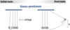 |
Fig. 2 Sketch depicting a Gauss pendulum. |
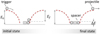 |
Fig. 3 Mixed metaphor diagram illustrating the process by which the projectile ball gains a kinetic energy ΔE over the initial kinetic energy of the trigger ball. |
2 Methods
While using the Gauss Pendulum setup, we aimed a more direct correlation between model, simulations and experimental data without anyloss in the rich physical phenomena involved with the Gauss rifle.
Furthermore, we propose a simple physical model for the gain in kinetic energy of the projected ball based on a magnetic potential well generated by the magnet. The main practical objective of this work is the corroboration of this model with simulations and experimental data using accessible laboratory equipment.
In this sense, we performed the following methodology:
-
In order to have a more direct comparison with the Gauss rifle, we accessed the performance of the Gauss pendulum with thenormal configuration, i.e., the elements being composed of steel balls and a magnet.
-
The magnetic potential well model has been evaluated experimentally using a set of hard polymer spacers in replacement of a steel ball in the setup. Measurements have been compared to simulated results.
Our first round of experiments (item 1) dealt with the normal configuration of the Gauss pendulum (Fig. 4). However, we soon realized that this particular set would limit our ability to address the magnetic energy potential well around the magnet. A second configuration has been developed by substituting the steel ball used as a spacer by a hard polymer spacer (item 2). As it is going to be explained later on, the usage of a set of polymer spacers with different thickness allowed us to address the depth and shape of the magnetic energy potential around the magnet.
The materials and important parameters used to build the Gauss pendulums are listed in Table 1.
After several different Gauss pendulum assemblies, testing different support sketches and tabletop setups, we ended up with the following configuration (see supplementary materials for images): two aluminum rods function as support for the set of 3 steel balls and a magnet suspended by 55 cm long wires. Each element was sustained by two wires, in the same fashion of most commercial Newton’s cradle toys, inducing a confined movement in a desired direction (plane). The set was assembled up against the window in order to improve the contrast of the movies taken from the shooting process and thus improving the precision while addressing the system.
Each trial has been filmed using a smartphone in slow-motion mode in order to precisely address the final height of the projectile ball [12]. A grid consisted of 5×5 cm2 square elements was painted on the window. Measurements were taken to account for parallax effects. The trigger ball has always been released with the swing angle smaller than 5° to guarantee that its initial energy was negligible.
In the second part (item 2), simulations and experimental procedures were performed in a rather intertwined manner and each incremental step is described in the results section.
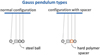 |
Fig. 4 Two distinct Gauss pendulum configurations tested in this work. The normal configuration uses a steel ball as a spacer, with the same functionality as the Gauss rifle depicted in Figure 1. The second configuration uses a hard polymer spacer instead of a steel ball. By doing so, we could easily manufacture several separators differing in thickness. |
Materials used to build the Gauss pendulum.
3 Results
3.1 Experiments with normal configuration of the Gauss pendulum
This configuration represents the direct conversion of the Gauss rifle into its pendulum form. After 10 trials the maximum height registered by the projectile ball was 30 (±1) cm. Assuming that the kinetic energy acquired the projectile ball after collision is transformed in gravitational potential energy by the swinging process of the pendulum, and considering that the initial kinetic and gravitational potential energy of the trigger ball is negligible, we ended having and energy gain of
 (1)
(1)
Studies of Gauss rifles available in the literature typically present the measured kinetic energy of the projectile ball in the range from 0.005 J [6] to 0.25 J [5]. This difference of almost two orders of magnitude can be attributed to variations in several relevant parameters such as magnet and ball sizes, number of stages, magnet fixture and so on. Nonetheless, our results comply fairly with the reported kinetic energy of the projectile ball in the literature. In order to continue with our Gauss pendulum study, we decided to perform further changes, departing from previously published Gauss rifle assemblies by substituting the spacer ball by tailored hard polymer specimens.
Another aspect worth noticing is that, in the shooting process, about 25% of the energy is transferred to the “magnet-spacer-trigger ball” system. This effect is evident while performing the experiment (see movie in supplementary materials). The mechanism of this energy transfer in not only due to the soliton recoil effect as described for Gauss rifles [2]. Note that before the collision, the system “magnet-spacer-projectile ball” is free to move and attracted magnetically to the trigger ball. When the collision happens, the system with the magnet is no longer at rest and the contact physics and energy transfer to the projectile ball happens with this new degree of freedom.
3.2 Experiments with the Gauss pendulum using polymer spacers
In this part of the experiment, the steel ball spacer has been replaced by a set of different hard polymer spacers in order to address the depth and shape of the magnetic energy well around the magnet. As a procedure, the energy of the projectile ball (maximum height) was measured as a function of the thickness of the spacer.
We machined an acrylonitrile butadiene styrene (ABS) specimen in order to get a set of 10 different spacers with thicknesses 1.10, 1.55, 2.00, 2.45, 3.00, 3.45, 4.00, 4.60, 5.15, 6.30 mm respectively.
We experimentally determined the coefficient of restitution (COR) between the polymer and steel balls to be 0.85(±0.04) [13]. The COR between a steel ball and a granite bench was also measured, resulting in the same value. However, the results were different for aluminum and iron surfaces. These results are consistent with the hypothesis that the kinetic energy is dissipated mainly within the steel balls in the case of collision with hard surfaces. Furthermore, it is reasonable to consider that the introductionof the polymer spacers will maintain the contact physics consistent with previous experiments with Gauss rifles. The COR determination between steel balls and the sintered magnets was not possible due to the strong magnetic interaction.
For each one of the 10 spacers, the Gauss pendulum was fired 3 times and the maximum height of the projectile ball was determined with a smartphone camera in the same method used in the previous experiment. For each set of 3 trials associated with one particular spacer, we assigned the maximum height as the yield of the system with such spacer. This methodology justifies the asymmetric error bars associated with the experimental dots as can be seen in Figure 13 (blue dots), along with the results of the simulations performed to validate the model of the magnetic energy well to explain the energy gain of the assembly. Looking at Figure 13 closely, it is noticeable that there is no height gain of the projectile ball for the thinnest spacer of 1.10 mm evidencing the unavoidable partial energy loss (inelastic collision) of the whole sequence of mechanical interactions. For the next four spacers, we see that the energy acquired by the projectile ball increases consistently with the model of the potential well depicted in Figure 3. Within the experimental error, the maximum height of the projectile ball (15 cm) happens for spacers between 3.45 and 4.60 mm. For broader spacers the maximum height tends do decrease indicating that other sources of energy loss come into play.
3.3 Simulations for the potential well for the Gauss pendulum with spacer
We aimed for the simplest model that explains the experimental results adequately. More specifically, we aimed for a model to calculate the final height of the projectile ball given a specific spacer. Furthermore, for the sake of a richer assessment, we modeled and analyzed not just energy profiles, but also the forces involved.
In order to use the experimental data to validate our model we performed the following steps:
-
We proposed a model by simulating the field distribution around the magnet and the steel balls as a function of the separation between them.
-
From the magnetic field model, we derived a model for the force of the interaction as a function of the separation.
-
The model for the force has been validated experimentally.
-
Taking into account the validated model of the force along with Newton’s law of mechanics and using the principle of energy conservation, we calculated the height of the projectile ball predicted for each spacer.
-
The results are compared with the experimental values.
Step 1 was based on a static model for forces between two magnets [14] as well as a model for interaction between soft magnetic particles in the presence of magnetic fields [15]. The magnetic interaction between the magnet, the trigger and projectile steel balls has been simulated using Finite Element Modeling Magnetics (FEMM) software [16] in order to address the forces between these elements and the kinetic energy gain of the projectile ball in relation to the trigger ball. After some trials with the calculations, the simulated parameters for the magnet have been chosen to be an intersection between NdFeB32 and NdFeB37 with polarization of 1.18 T. Since the steel balls are engineered for their mechanical properties, modeling their magnetic properties is challenging due to their inherent inhomogeneity. As a fair approximation we used the pure iron properties listed within FEMM software. The simulated magnetic properties of the polymer spacers were considered to be the same as vacuum.
Figure 5 shows the resulting simulations for the magnetic field distribution of the system “trigger ball-magnet-projectile ball” in two different conditions.
We considered 4 different configurations while simulating the shooting process of the Gauss Pendulum: no spacer, 2, 3 and 4 mm spacer. For each configuration, the whole process has been simulated statically considering a sequence of 80 steps, each representinga 0.02 mm variation of the distance of the trigger ball (before the collision), or projectile ball (after the collision) from the magnet. From each simulated step we calculated the magnetic energy of the system in such condition. The results of the simulation are presented in Figure 6 in a similar way we presented the pictorial model in Figure 3. However, to interpret Figure 6, we have to introduce several subtleties in its representation.
The left portion of Figure 6, where distances are negative, represents the space where the trigger ball approaches the magnet. In the same sense, positive distances represent the separation between the projectile ball and the magnet. Note that the magnet has no space dimension in this representation.
Figure 6 can be seen as if time flows from the left, when the trigger ball is far and rolling towards the magnet, to right, as the projectile ball moves away from the magnet. Note that the final energy in all configurations is the same (0.202 J), as all configurations end with the same condition, i.e.: the trigger ball attached to the magnet and the projectile ball far from it.
The main subtlety of this representation is that the starting energy of each configuration is different. This can be understood easily once it is realized that the minimum energy of the system happens when the two steel balls are attached to the magnet (Fig. 5a). Thus, considering the first configuration with no spacer, the approachingprocess of the trigger ball is symmetric to the departure of the projectile ball and the later ends up with negligible velocity as the initial state of the former. Once you take into account energy dissipation (not considered in this stage of the model) one can understand why the Gauss Pendulum (or the rifle) does not work experimentally without a spacer. The simulation for the 2 mm spacer configuration starts with a higher magnetic energy when compared with the no spacer configuration. This is so because, in the initial condition, the projectile ball is separated 2 mm from the magnet, being out of the minimum energy condition. This renders the potential well in which the trigger ball falls higher than the potential well to be overcome by the projectile ball. The energy difference between the initial and final condition is highlighted in Figure 6 by the green band where ΔE = 0.019J. For the same reason, configurations with 3 and 4 mm spacers generate even higher energy differences, with values ΔE = 0.024J and ΔE = 0.027J respectively.These results are consistent with the energy of the projectile ball obtained in section III.A. If no energy losses were present, this energy difference would be converted in kinetic energy of the projectile ball at the end of the process.
Other general conclusions can be taken from Figure 6. Note that more than half of the magnetic potential well energy is situated within 2 mm distance from the magnet. This justifies substituting the traditional steel ball spacer by thinner polymer spacers in order to address the magnetic potential well around the magnet and better understand the workings of the Gauss pendulums and rifles. Furthermore, although the absolute values are quite different, the general shapes of the potential wells are very similar, indicating that the forces (derivatives of the potentials) are essentially the same for a given distance. For the sake of better comparison, in Figure 7 we plot the potential felt by the trigger ball for each configuration, where we collapsed all the curves to zero final energy. Based on the similarity of the curves, we considered that the force felt by the trigger ball as a function of the distance is independent of the configuration (spacer thickness) of the projectile ball on the opposite side of the magnet. The exponential behavior of the potential curves is evident by the straight progression of all four curves in the inset, where energy axis is set in logarithmic scale.
Based on the FEMM simulations we estimated the behavior of the force exerted by the magnet on the steel balls as a function of the distance and validated such estimative experimentally as can be seen in Figure 8. The model depicted by the red line is the derivative of the magnetic energy potential shown in Figure 7 (red line). To validate this model we measured experimentally, using a setup sketched in Figure 9. The magnet was held fixed to a support bar up to a certain height. Also with the use of a strap, a steel ball was kept fixed to a bucket and attached to the magnet with a polymer spacer in between in such a way that the bucket was hanging with the bottom just about 1 cm from the floor. Next, water was slowly and gently (avoiding impulse contributions) introduced in the bucket in order to attain a slow increase of the mass in the bucket. This process was continued until the bucket fell on the floor, indicating that the weight force became vanishingly higher than the force between the magnet and the steel ball. After each such trial the weight of the system “bucket strap steel ball” was measured with a balance. For each spacer we performed 5such procedures and the corresponding values are plotted in Figure 8 as the experimental values.
The measured and modeled values for the force present a legit agreement, showing a fair quantitative correspondence, and the same qualitative behavior evidenced here in the logarithmic scale. The rather minor systematic difference between model and experimental values can be attributed in small part to the approximations in the magnetic parameters fed into the calculations, and in major part to the well known limitation of the usage of first order finite element calculations in non linear interfaces such as magnet/air/steel balls [17].
After the simulated forces have been validated experimentally we devised a model to predict the final height of the projectile ball after the shooting process for each spacer.
This model has been implemented using Scilab software [18]. The Gauss pendulum is separated in two pieces: the trigger ball and the set formed by the magnet, spacer and projectile ball. The important physical parameters are the length of the pendulum (L), the swinging angle of the trigger ball (θ1) and the “magnet spacer projectile ball” (θ2), the linear separation between the pieces from rest position (x), the magnetic force of interaction (Fmag), and the masses and weight forces of each piece (M1, M2, w1, w2), as indicated in Figure 10. The physical model considers that the magnetic force generates a torque in each piece given by:
![Mathematical equation: \begin{equation*}T_{mag}=F_{mag} L\left[[cos\left(\frac{\theta_1+\theta_2}{2}\right)\right] \end{equation*}](/articles/emsci/full_html/2021/01/emsci200008/emsci200008-eq2.png) (2)
(2)
The weight force component perpendicular to the direction of the wire for each individual piece is also taken into account as a contributionto the total torque (T). The acceleration of each piece was calculated using Newton’s relation for torque and moment of inertia (J):
 (3)
(3)
where ω is the angular speed. Once the values for the accelerations are determined and using the measured values for the masses of each component, we used Euler’s numerical integration method in order to determine new positions for each iteration step in the simulation. Each iteration corresponds to 1 microsecond.
The simulation followed the algorithm shown in Figure 11. The initial value for θ1 has been set to 2°, guaranteeing a negligible energy to the trigger ball. There is a subtle moment in the calculations regarding the collision process. In this moment, a coefficient of restitution COR = 0.85 (evaluated experimentally) is attributed to the interaction between the trigger ball and the system “magnet spacer projectile ball”. The uncertainty has been suitably evaluated considering the complex dynamics of the collision, involving a sequence of steel balls, magnet and polymer spacer.
As a result of this interaction, the trigger ball ends up attached to the magnet and the projectile ball is shot forward. For the simulations, the process results in an “inversion of the pieces” leaving a piece composed by the trigger “ball magnet spacer” on the side once occupied by the sole trigger ball, and a sole projectile ball on the other.
As already discussed in the context of Figure 6, the presence of the spacer renders the potential well felt by the projectile ball to be uneven symmetrically when compared to the approximation of the trigger ball. All this is taken into account in the simulation in order to calculate the final height reached by the projectile ball during its pendulous motion.
In Figure 12 we can observe the results of the simulation for a 2 mm spacer, namely the height, angular speed and total energy of each peace as a function of time. Similar simulations have been performed for several different spacer thicknesses. In the first layer, the height of the projectile ball and the system trigger “ball magnet spacer” is shown as a function of time. Note that the latter (blue line) suffers recoil in the interaction, moving up to 1.7 cm in the height scale. The projectile ball is ejected with high kinetic energy, reaching 11.3 cm height. This value can be checked with the simulated value (red line) in Figure 13 for 0.002 mm spacer. Analyzing Figure 12 further, on the second layer we show the simulated values for the angular speed for both pieces as a function of time, where a sharp peak is noticeable in both cases in the collision moment. The sharpness of these peaks is the result of an artifice introduced in the model in order to account for the energy dissipation in the moment of the collision, approaching the model to experimental evaluation of the coefficient of restitution of 0.85 in the collisionbetween magnet and steel ball. This energy dissipation is the responsible for the sudden decrease in the total energy of the system at the moment of collision visible in the third layer of Figure 12.
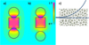 |
Fig. 5 FEMM simulations of the magnetic field distribution of the system for two different configurations: (a) minimum energy and (b) projectile ball separated 4 mm from the magnet. Scale units are represented as magnetic induction intensity (B) measured in Tesla (T). (c) Mesh distribution in the region around the point contact between the magnet and the steel ball. |
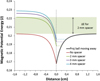 |
Fig. 6 Finite Element Method Magnetic (FEMM) simulation for the magnetic energy considering four different configurations of the Gauss Pendulum shooting process: no spacer, 2, 3 and 4 mm hard polymer spacers. |
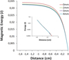 |
Fig. 7 Potential felt by the trigger ball for each configuration identified by the spacer thickness, where we collapsed all the curves to zero final energy. The exponential behavior of the potential curves is evident by the straight progression of all four curves in the inset, where energy axis is set in logarithmic scale. |
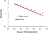 |
Fig. 8 Forceexerted by the magnet on the steel ball as a function of separation. The model is obtained from the derivative of the potential well function (Figure 7 red line). Experimental data obtained by an experimental procedure is described in Figure 9. The straight line in the log scale in both cases evidences the quadratic nature of the interaction. |
 |
Fig. 9 Sketch of the apparatus used to determine experimentally the force between the magnet and a steel ball as a function of the separation. The amount of water was increased slowly and gently until the weight of the system bucket_ strap_steel ball surpassed the magnetic interaction of the ball with the magnet. After each trial the weight was determined with a balance. |
 |
Fig. 10 Sketch of the Gauss pendulum indicating relevant parameters for the Scilab model simulations. |
 |
Fig. 11 Algorithm used in the Scilab simulation in order to calculate the final height of the projectile ball for a series of shooting process, which differed by spacer thickness. |
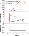 |
Fig. 12 Scilab simulations for height, angular velocity (for each part of the pendulum identified in the caption) and total energy as a function of time for the case of the 2 mm spacer. |
 |
Fig. 13 Experimental and simulated results for the final height reached by the projectile ball as a function of the thickness of the spacer. |
4 Discussion
The results described in subsections B and C are shown together in Figure 13. The experimental and simulated results present a remarkable qualitative match. As the height of the projectile ball is proportional to the energy gain, Figure 13 can be seen as an assessment of the magnetic energy potential as a function of the distance from the magnet.
The relevance of this result is enhanced once we take into account that potential wells are so often discussed in physics. However, for the fundamental forces, only the magnetic interaction is measurable in standard laboratory infrastructure, as the electric, nuclear and gravitational effect variations happen in scales that are too big or too small requiring sophisticated or expensive setups. In the literature of Gauss rifles, magnetic potential wells are treated by analogy [11]. Other works focused their analysis on field and forces [2,6,7].
The fact that the experimental results are systematically smaller than the simulated ones is reasonable and expected. This evidences that there are more energy losses than just the inelastic fraction of the collision process taken into account in the model.
5 Dead end
This work started about the Gauss rifle in the context of the educational material prepared by our group in 2017 [3]. In order to improve on the existing literature, we tried to address the role of dissipative phenomena such as rolling and sliding friction of the balls on the rail. Several videos have been recorded of the Gauss rifle shooting with marked balls with the purpose of determining the rotation of the balls along the whole process. By doing this, we aimed to have better agreement between experimental and calculated values for the magnetic potential. Such procedure ended up being more cumbersome than initially thought. Similar problems have been reported by other authors [6,7] and we came to know about their experience after our trials. In the effort of avoiding or isolating the friction forces, we came up with the idea of the Gauss pendulum.
6 Conclusions
We proposed the Gauss pendulum, an experimental setup simpler than the Gauss rifle, which gives new opportunities for assessing and modeling magnetic interactions. We demonstrated advantages of the Gauss pendulum, since it avoids the hard question regarding the energy partition in terms of translation and rotation of the balls used in the Gauss rifle setup. The usage of polymer separators allowed the experimental evaluation of the magnetic potential using two different techniques. We demonstrated remarkable correlation between the magnetic potential well model, simulations and experimental data.
Supplementary Material
Supplementary file supplied by the authors. Access Supplementary Material
Acknowledgements
The authors would like to thank prof. Gerson Mantovani for providing us the ABS specimen and Adinan Brito for assisting us with video editing.
References
- US Navy Railgun – Their Most Powerful Cannon (2018), Access in December, 2020 [Google Scholar]
- A. Chemin, P. Besserve, A. Caussarieu, N. Taberlet, N. Plihon, Am. J. Phys. 85, 495 (2017) [CrossRef] [Google Scholar]
- J. Schoenmaker, J.C. Teixeira, Rifle de Gauss. BasesConceituais da Energia. [Google Scholar]
- The magnetic cannon (gauss gun) was one of the 17problems selected for the 8th edition of the InternationalPhysicists’ Tournament [Google Scholar]
- J. Rabchuk, Phys. Teacher 41, 158–161 (2003) [Google Scholar]
- Andersson, C.-J. Karlsson, H. Lane, Emerg. Sci. 1, 6 (2017) [Google Scholar]
- G. Magkos, B. Gabritchidze, K. Patatoukos, Emerg. Sci. 1, 4 (2017) [Google Scholar]
- Measurements of this paper and above references showthat the contact magnetic forces are on the order of 2N.The friction force we are speaking about is a fraction of the weight force, on the order of 0.05N [Google Scholar]
- S. Hutzler, G. Delaney, D. Weaire, F. Macleod, Am. J. Phys. 72, 1508 (2004) [CrossRef] [Google Scholar]
- C. Gauld, Sci. Educ. 15, 597 (2006) [Google Scholar]
- L.A. Elliott, A. Bolliou, H. Irving, D. Jackson, Phys. Teacher 57, 520 (2019) [Google Scholar]
- We used an iPhone6 in slow motion mode, which shoots 240 frames per second. A selected trial can be seen in the supplementary materials [Google Scholar]
- N. Farkas, R. Ramsier, Phys. Educ. 41, 73 (2005) [Google Scholar]
- D. Vokoun, M. Beleggia, L. Heller, P. Sittner, J. Magn. Magn. Mater. 321, 3758 (2009) [CrossRef] [Google Scholar]
- A. Mehdizadeh, R. Mei, J.F. Klausner, N. Rahmatian, Acta Mech. Sin. 26, 921 (2010) [Google Scholar]
- D. Meeker, Finite Element Method Magnetics, Version4.2, User’s Manual (2019) [Google Scholar]
- R. Pile, E. devillers, J. Le Besnerais, IEEE Trans. Magn. 54, 1 (2018) [CrossRef] [Google Scholar]
- Scilab website, Accessin October 2019 [Google Scholar]
Cite this article as: Julio Carlos Teixeira, Pâmella Gonçalves Martins, Amanda Schwartzmann, and Jeroen Schoenmaker. The Gauss pendulum, Emergent Scientist 5, 3 (2021)
All Tables
All Figures
|
Fig. 1 Sketch depicting a Gauss rifle. |
| In the text | |
|
Fig. 2 Sketch depicting a Gauss pendulum. |
| In the text | |
|
Fig. 3 Mixed metaphor diagram illustrating the process by which the projectile ball gains a kinetic energy ΔE over the initial kinetic energy of the trigger ball. |
| In the text | |
|
Fig. 4 Two distinct Gauss pendulum configurations tested in this work. The normal configuration uses a steel ball as a spacer, with the same functionality as the Gauss rifle depicted in Figure 1. The second configuration uses a hard polymer spacer instead of a steel ball. By doing so, we could easily manufacture several separators differing in thickness. |
| In the text | |
|
Fig. 5 FEMM simulations of the magnetic field distribution of the system for two different configurations: (a) minimum energy and (b) projectile ball separated 4 mm from the magnet. Scale units are represented as magnetic induction intensity (B) measured in Tesla (T). (c) Mesh distribution in the region around the point contact between the magnet and the steel ball. |
| In the text | |
|
Fig. 6 Finite Element Method Magnetic (FEMM) simulation for the magnetic energy considering four different configurations of the Gauss Pendulum shooting process: no spacer, 2, 3 and 4 mm hard polymer spacers. |
| In the text | |
|
Fig. 7 Potential felt by the trigger ball for each configuration identified by the spacer thickness, where we collapsed all the curves to zero final energy. The exponential behavior of the potential curves is evident by the straight progression of all four curves in the inset, where energy axis is set in logarithmic scale. |
| In the text | |
|
Fig. 8 Forceexerted by the magnet on the steel ball as a function of separation. The model is obtained from the derivative of the potential well function (Figure 7 red line). Experimental data obtained by an experimental procedure is described in Figure 9. The straight line in the log scale in both cases evidences the quadratic nature of the interaction. |
| In the text | |
|
Fig. 9 Sketch of the apparatus used to determine experimentally the force between the magnet and a steel ball as a function of the separation. The amount of water was increased slowly and gently until the weight of the system bucket_ strap_steel ball surpassed the magnetic interaction of the ball with the magnet. After each trial the weight was determined with a balance. |
| In the text | |
|
Fig. 10 Sketch of the Gauss pendulum indicating relevant parameters for the Scilab model simulations. |
| In the text | |
|
Fig. 11 Algorithm used in the Scilab simulation in order to calculate the final height of the projectile ball for a series of shooting process, which differed by spacer thickness. |
| In the text | |
|
Fig. 12 Scilab simulations for height, angular velocity (for each part of the pendulum identified in the caption) and total energy as a function of time for the case of the 2 mm spacer. |
| In the text | |
|
Fig. 13 Experimental and simulated results for the final height reached by the projectile ball as a function of the thickness of the spacer. |
| In the text | |
Current usage metrics show cumulative count of Article Views (full-text article views including HTML views, PDF and ePub downloads, according to the available data) and Abstracts Views on Vision4Press platform.
Data correspond to usage on the plateform after 2015. The current usage metrics is available 48-96 hours after online publication and is updated daily on week days.
Initial download of the metrics may take a while.