| Issue |
Emergent Scientist
Volume 1, 2017
International Physicists' Tournament 2016
|
|
|---|---|---|
| Article Number | 4 | |
| Number of page(s) | 8 | |
| DOI | https://doi.org/10.1051/emsci/2017004 | |
| Published online | 01 September 2017 | |
Research Article
Testing a simple model for the magnetic cannon
University of Crete, Physics Department,
Heraklion, Greece
* e-mail: This email address is being protected from spambots. You need JavaScript enabled to view it.
Received:
19
December
2016
Accepted:
11
July
2017
Abstract
A magnetic cannon consists of a line of steel balls which are in contact with a permanent magnet. If another steel ball collides with the system on one side, then the ball at the other end of the line is ejected at high speed. A theoretical model is proposed for the system by neglecting energy losses and making the approximation that the magnetic field is uniform near each ball. Our model can account for any magnet shape and is able to accurately predict the most efficient system configuration, as verified by experiments. Additionally, the predicted values of the ejection velocity are in most cases found to be in reasonable agreement with the experiment.
Key words: Gauss rifle / Gaussian accelerator / magnetism / energy conservation / measurement of velocity
© G. Magkos et al., Published by EDP Sciences, 2017
 This is an Open Access article distributed under the terms of the Creative Commons Attribution License (http://creativecommons.org/licenses/by/4.0), which permits unrestricted use, distribution, and reproduction in any medium, provided the original work is properly cited.
1 Introduction
The magnetic cannon is a simple system that behaves in an unintuitive way. It consists of a line of steel balls, which is placed in contact with a permanent magnet. When another steel ball, initially at rest, is released under the attraction of the magnet, it collides with the line of balls and magnet. Then, the final ball in the line is ejected with a surprisingly high velocity. A sketch of the system is shown in Figure 1. At first glance, because the velocity of the ejected ball is much higher than that of the incoming ball, this system appears not to respect the law of conservation of energy. With a closer look, however, the reason for this surprising behaviour is clear: the potential energy of the system is significantly reduced when the incoming ball reaches the line of balls, thus allowing for a substantial increase in kinetic energy.
Although relatively simple, this system allows one to study the laws of physics related to magnetism, collision dynamics and classical mechanics. It has often been used by physics teachers in order to acquaint their students with basic principles like energy conservation.
Several papers on the magnetic cannon have been published, primarily from such a point of view. Rabchuk [1] presented a method of measuring the kinetic energy of the incoming and ejected ball and calculated the changes in potential energy during the motion of the ball using a finite element magnetics software. Kagan [2], as well as Ucke and Schlichting [3], used a different method to measure both the kinetic and potential energy differences and obtained an estimate for the energy losses in the system. Finally, McDonald [4] presented a simple model for estimating the velocity of the ejected ball.
In the present work, the model of reference [4] is extended to treat magnets of different shapes, and its validity is examined by comparing its predictions for the velocity of the ejected ball with experimental results using different magnets and initial configurations. While the model contains several simplifying assumptions, such as neglecting energy losses, a reasonable agreement is in most cases still found.
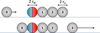 |
Fig. 1 A sketch of our system. Red and blue colours depict the poles of the magnet. An incoming ball collides with the line of balls and magnet, and the final ball in the line is ejected with high velocity. |
2 Methods
2.1 Experimental setup
For our experiment, neodymium magnets of different shapes (rectangular, cylindrical and spherical, with two different sizes for the rectangular magnets) and steel balls of two different sizes were used. The balls were free to roll on an aluminium (non-magnetic) rail to ensure rectilinear motion. The magnet was held in place using tape, in order to restrict its backward motion when the incoming ball approaches, so as to maximize the velocity of the final ball. The cannon was placed near the edge of the rail to minimize friction.
The velocity was measured by allowing the final ball to freely fall from the edge of the rail (placed on a specific height h from the ground) and measuring the horizontal distance x it traversed until it reached the ground (x is also called the range of the projectile). Therefore, neglecting the effects of air resistance, the final velocity was:
 (1)
where g is the gravitational acceleration.
(1)
where g is the gravitational acceleration.
2.2 Measurements of system parameters
Our theoretical calculations depended on the following system properties: the size of the magnets and balls, the mass of the balls and the magnetic field strength of each magnet as a function of distance from its center.
The required sizes and masses of the magnets and balls are shown in Table 1. The larger balls were used only with the large rectangular magnet and the smaller balls only with the other magnets.
Using a Hall sensor, the magnetic field of the large rectangular magnet was measured as a function of the distance from its center along the line parallel to the magnetization. For the rest of the magnets, the magnetic field was measured for a few values of distance from their center.
Magnet and ball dimensions and ball masses. The side of the magnet that is parallel to the line of balls and the magnetization is denoted 2r.
2.3 Energy losses
Energy losses were estimated by measuring the potential energy difference for a single initial configuration and comparing it with the kinetic energy of the ejected ball. The method used was similar to the one presented in references [2,3]. The potential energy difference is equal (in absolute magnitude) to the work done on the incoming ball minus that on the ejected ball. The work was calculated by measuring in each case the force exerted on the ball as a function of distance. The measurement was carried out by gluing a rope on the ball, passing the rope through a pulley, and using weights to determine when the ball would fall. The distance between the ball and the cannon was adjusted by placing paper sheets of known thickness in between. The resulting relations of force as a function of distance were then numerically integrated using the trapezoid rule to arrive at the final value of the potential energy difference.
2.4 Theoretical work
A line of steel balls of mass m, radius r0 and relative permeability μr is placed along the x-axis. A magnet of length 2rM is placed at some position in the line in between the balls, defining in this way a specific configuration (for example 0 balls on the left hand side (LHS) and 3 balls on the right hand side (RHS) of the magnet). Another identical steel ball with negligible initial velocity, moves along the x-axis towards the LHS of the magnet, and collides with the line. If it is energetically allowed, the final ball on the RHS will be ejected at a high velocity. After the ball is ejected, the system now has a different configuration (for example 1 ball on the LHS, and 2 balls on the RHS). Our aim is to calculate the velocity of the final ball and examine its dependence on system parameters.
Neglecting the initial kinetic energy and any energy losses during the collision or due to friction, the final kinetic energy Kf will be equal to the difference between the potential energies of the initial (Ui ) and the final configuration (Uf).
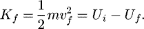 (2)
(2)
Therefore the final velocity will be:
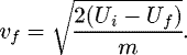 (3)
(3)
The problem is then reduced to calculating the potential energy for the initial and final configuration. The potential energy depends on the magnetic field of the permanent magnet. A way to derive expressions for the magnetic field of different magnets is presented in the following section.
2.5 Magnetic field
The magnetic field at a position r of a dipole with dipole moment p placed at the origin of the coordinate system is
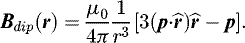 (4)
(4)
For a magnet of any shape with magnetization M(r), the magnetic field then is:
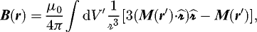 (5)
where the integration is over the volume V of the magnet, r′ is the position vector of each point of the magnet, and
(5)
where the integration is over the volume V of the magnet, r′ is the position vector of each point of the magnet, and  .
.
Equation (5) indicates that the magnetic field depends on the shape of the magnet. For each magnet shape that was used in our experiment (rectangular, cylindrical and spherical), expressions for the magnetic field were derived under the assumption that each magnet has a uniform magnetization M. The resulting integrals were then computed numerically, given the dimensions of the magnet, the magnetization and the desired position. The magnetization was specified by computing the above integral for a specific position relative to the magnet, and measuring the magnetic field of our magnet for the same position.
For a spherical magnet, the situation is simpler. It is known [5] that the magnetic field outside a sphere of uniform magnetization M and radius R is the same as the magnetic field of a dipole with moment  , which is given by equation (4).
As will be shown below, for our theoretical calculations it is necessary to know only how the magnetic field behaves at some distance from the center of the magnet along the axis of magnetization, which is where the steel balls are placed in our model.
2.6 Calculating the final velocity
Given the magnetic field of the magnet, our goal is now to determine how the magnet influences the line of steel balls, how the magnetized steel balls influence each other, and finally to calculate the potential energy of any configuration of interest.
First, it is needed to determine how a single ball is affected by a magnetic field. As a simplification to the problem, the magnetic field near each sphere is taken to be uniform. The value of the magnetic field is taken to be the same as that at the center of the sphere. Essentially, in this simplification, the magnetic field is considered to not change significantly in the vicinity of the sphere. This approximation is in general more valid as the sphere becomes smaller, and as the distance from the magnet becomes larger. The validity of this approximation also depends on the exact way that the field scales with distance, which in turn depends on the shape of the magnet. The approximation is not expected to be perfectly valid in our system and is meant to simplify the problem.
When a permeable sphere of permeability μ is placed in a uniform magnetic field B0, it takes on a uniform magnetization, and a sphere of uniform magnetization produces, as mentioned before, the magnetic field of a dipole outside the sphere.
The total magnetic field B = μH can, in regions of uniform permeability, be derived from a scalar potential Φ such that H = −∇Φ, which obeys the Laplace equation ∇2Φ = 0. Requiring that Φ is zero at infinity, finite at the origin and continuous on the surface of the sphere, after some calculations it is found that the induced dipole moment of the sphere is:
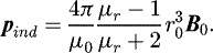 (6)
(6)
If μr ≫ 1 (for steel with ferromagnetic properties, this certainly holds [6]), then this formula simplifies to:
 (7)
(7)
The sphere behaves as a dipole, so its induced magnetic field will be given by equation (4). If only the magnetic field on the axis of magnetization (which is in our setup where the line of balls is placed) is needed, then this formula becomes:
 (8)
(8)
Our next step is to determine the induced dipole moment of every ball in a specific configuration. It is now necessary to take into account both the interaction of every ball with the magnet and that of every ball with each other. The configuration with 0 balls on the LHS and 3 balls on the RHS of the magnet, which is presented in Figure 1, is used as an example. For simplicity, our magnet is assumed to be spherical with uniform magnetization, and thus to behave as a dipole with dipole moment p. For a magnet of different shape, to calculate its magnetic field, an integral of the form of equation (5) needs to be computed. If pi is defined as the induced dipole moment of the ith ball closer to the magnet, and Bi as the value of the magnetic field at its center, then the following system of equations needs to be solved:
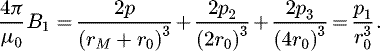 (9)
(9)
 (10)
(10)
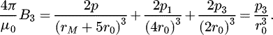 (11)
(11)
By solving this system, p1, p2 and p3 can be found in terms of p, r0 and rM .
Now, it is possible to calculate the potential energy of the configuration, by using the formula
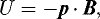 (12)
which describes the magnetic potential energy of a magnetic dipole of moment p placed in a magnetic field B. Again, it is assumed that the magnetic field is uniform in the vicinity of the sphere.
(12)
which describes the magnetic potential energy of a magnetic dipole of moment p placed in a magnetic field B. Again, it is assumed that the magnetic field is uniform in the vicinity of the sphere.
For our configuration:
 (13)
where the terms with index Mi correspond to the magnetic energy of the ith ball due to its presence in the magnetic field of the magnet and the terms with index ij correspond to the magnetic energy of the interaction between two of the steel balls.
(13)
where the terms with index Mi correspond to the magnetic energy of the ith ball due to its presence in the magnetic field of the magnet and the terms with index ij correspond to the magnetic energy of the interaction between two of the steel balls.
Using equation (12), (13) becomes:
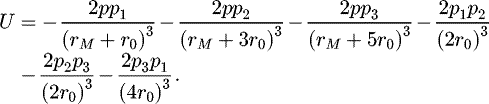 (14)
(14)
To examine the transition from this configuration to that with 1 ball on the LHS and 2 on the RHS, the potential energy for the other configuration can also be calculated in the same way, and then, by inserting our results to equation (3), the velocity of the final ball after it is ejected can be found.
The potential energy and the final velocity for all configurations with up to a total number of 5 balls have been calculated given the parameters of our experiment. For some initial configurations (e.g. 1 ball on the LHS of the magnet and 2 on the RHS) the final ball is not ejected, because the difference in potential energy of the initial and final configuration is less than or equal to zero.
The final velocity has also been calculated for the same configurations for magnets of different shapes that were used in our experiment. There, the calculation was more complicated, because the magnetic field of the magnets was computed numerically from equation (5), given the parameters of our magnets.
The results of our theoretical calculations are presented in Section 3, where they are compared with the outcome of our experiment.
3 Results
3.1 Magnetic field
First, our theoretical and experimental results for the magnetic field of the large rectangular magnet are presented and compared. The results are given in Figure 2. The main panel shows the magnetic field of the magnet as a function of distance from its center. The inset shows the same dependence in a logarithmic plot.
The theoretical values were calculated with equation (5), by using the experimental value at a distance of 0.5 cm from the surface of the magnet (or 0.9 cm from its center) to calculate the parameter M.
To verify that choosing an arbitrary point to calculate M does not significantly affect the value of M more than the error would allow, the standard deviation of the values of M calculated for each point of up to a distance of 1 cm from the surface of the magnet was computed and compared with the error for each point derived from error propagation given the error of B. It was found that the error derived from error propagation is for all points comparable with the standard deviation and in some cases larger. Therefore, the precision of the value of M is not significantly affected.
Good agreement is observed between the theoretical and experimental values, especially for smaller to intermediate distances. For larger distances it can be seen (Fig. 2, inset) that the theoretical and experimental results scale slightly differently, although the actual values of the magnetic field (Fig. 2, main panel) are still quite similar so that using the theoretical values for our calculations does not significantly affect our results. Also, the two values for the distances closest to the magnet are not in very good agreement with theory. These discrepancies could mean that our assumption of homogeneous magnetization is not perfectly valid, and it is expected to break down especially at small distances from the magnet.
It should be noted that the magnetic field scales less rapidly than 1/r3, for both the theoretical and experimental values. At larger distances than those included in Fig. 2, where the far-field limit is reached, the magnetic field is naturally expected to decay as 1/r3.
For all the magnets, the magnetic field measurement that was used to calculate the magnetization M, and the value of the magnetization M that was found are presented in Table 2. All measurements were made at a distance of 0.50 ± 0.05 cm from the surface of the magnet.
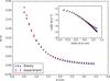 |
Fig. 2 Main panel: The magnetic field of the large rectangular magnet as a function of distance from its center. The red points show the experimental values and the blue points the theoretical values. Inset: The same dependence in a logarithmic plot. The theoretical values were calculated numerically by using the experimental value at d = 0.9 cm to determine the magnetization of the magnet, considered homogeneous. The validity of this approach is discussed in the text. |
The magnetic field B that was measured for each magnet at a distance of 0.5 cm from its surface, as well as the magnetization M that was calculated from it.
3.2 Most efficient configuration
Here our theoretical and experimental results for the velocity of the final ball are presented for different initial configurations. The results for all of our magnets are shown in Figure 3.
The configuration 0 + 2 means that initially there are 0 balls on the LHS of the magnet and 2 balls on the RHS. The configurations that are not included for up to a total number of 5 balls, e.g. 1 + 2 or 2 + 2, do not cause the ejection of the final ball. The reason for that is that the potential energy of the initial configuration is greater than or equal to that of the final configuration, and thus it is not energetically allowed for the final ball to gain kinetic energy.
The error of the experimental values is about 3 cm/s. This was determined by taking the standard deviation of the velocity for 5 measurements. This value is about the same as or greater than the error derived from equation (1) using error propagation.
For all magnets, the most efficient initial configuration for a given number of balls N (where N ≤ 5) is that which has 0 balls on the LHS and N balls on the RHS. This is agreed on both by theory (blue points, Fig. 3) and experiment (red points, Fig. 3). For configurations with 1 ball on the LHS, the final ball is ejected with much less velocity, while for configurations with more than 1 ball on the LHS, the final ball is not ejected at all, at least for the total number of balls being up to 5.
Although the above trend for the most efficient configuration has only been experimentally confirmed for up to 5 balls, our model and intuition suggest that it will continue to hold for all N.
For the small rectangular magnet (first panel, Fig. 3), the theoretical values are, as expected, somewhat larger than the experimental, as they do not account for energy losses. It can be seen that the difference between the theoretical and experimental values is about the same for all configurations, which probably shows that the energy losses are also about the same. It should be noted that the measurements for the initial configurations with 1 ball on the LHS slightly deviate from this pattern.
For the large rectangular magnet (second panel, Fig. 3), a similar pattern to the small rectangular one can be seen. Also, in this case, as more balls are added to the RHS, the experimental value of the final velocity starts to decrease. The configuration that produces the maximum velocity has 0 balls on the LHS and 3 balls on the RHS. This means that for this system energy losses are larger, as would be reasonable, because the scale of the system is also larger.
For the cylindrical magnet (third panel, Fig. 3), the theoretical and experimental results are very close, except for the configurations with 1 ball on the LHS. However, some theoretical results are actually slightly smaller than the experimental, while our theory would be expected to always predict larger values than the experiment. Some possible reasons for this will be mentioned in Section 4.
Finally, for the spherical magnet (fourth panel, Fig. 3), most of the theoretical results are much smaller than the experimental. To some extent, this could be because for the spherical magnet our measurements of the magnetic field had much more uncertainty, as it was difficult to find where its poles were and to keep the magnet exactly aligned so that its poles faced our Hall sensor. This uncertainty in the magnetic field could have influenced our theoretical predictions. Also, at a distance of about 1.0–1.5 cm, the magnetic field was found to scale as 1/rx where x = 2.76 ± 0.25. Even though our measurements are not precise enough to verify it, the magnetic field might not scale exactly as 1/r3 , as would happen for a dipole. This would mean that the magnetization M is not exactly uniform, as has been assumed.
After finding that the optimal configuration for a given number of balls is, at least for up to 5 balls, that with all the balls on the RHS, an attempt was made to examine what the optimal number of balls is to achieve maximum velocity. However, it was not possible to make measurements for configurations with 6 or more balls, because it was observed that often more than one ball were ejected, and therefore a general answer to this question has not been found.
It is possible to say that the optimal number of balls has been found if, as the number of balls increases, the velocity of the final ball reaches a plateau and then starts to decrease. For the configurations that were tested, a decrease was observed only for the large rectangular and the cylindrical magnets. For the cylindrical magnet, though, the difference of velocities is within the error, and thus it is not certain if the optimal number has been found. For the large rectangular magnet, the optimal number of balls on the RHS is either 3 or 4, but most likely 3 (the difference between the corresponding velocities is within the error).
 |
Fig. 3 The final velocity for each of our magnets and for initial configurations with up to a total number of 5 balls. The blue points are the theoretical values and the red points the experimental values. |
3.3 Energy losses
For our chosen configuration (0 + 3, using the large rectangular magnet), the work done on the incoming ball as it approaches was found to be Wi = 40.7 mJ and on the ejected ball Wf = 2.2 mJ. The potential energy difference then is ΔU = 38.5 mJ. The kinetic energy measured in our experiment for this initial configuration is K = 32.8 mJ. Therefore the energy dissipated is Q = ΔU − K = 5.7 mJ, which is about 14.8% of the potential energy difference.
4 Discussion
4.1 Theoretical assumptions
First, a comment needs to be made on why two terms in the conservation of energy in equation (2), the initial kinetic energy, and the rotational energy, were neglected.
The initial kinetic energy was neglected because in our experiment the initial velocity of the incoming ball was quite small. For our large balls and typical initial and final velocities vi = 10 cm/s, vf = 200 cm/s, the respective kinetic energies are Ki = 4.5 × 10⁻⁵ J and Kf = 1.8 × 10⁻² J, the initial kinetic energy being 400 times smaller than the final.
The initial rotational energy  , where
  the moment of inertia of the ball, is even smaller than the initial translational kinetic energy and can safely be neglected. Here the ball is assumed to initially be rolling without slipping. The final ball is not expected to gain much rotational energy for our setup because it starts its motion with no rotation and stays on the rail for very little distance.
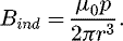
However, it is also necessary to check how much rotational energy is transferred to the incoming ball until it reaches the magnet, as this energy is not transferred to the final ball. For simplicity, our magnet is assumed to be spherical and can be treated as a dipole with moment p. The magnetic field then at a distance d from its center is Bmagn = μ0p/(2πd3). A steel ball approaching the magnet has an induced dipole moment given by equation (7), which produces a magnetic field given in equation (8). The force between the two dipoles is  . For our spherical magnet and small steel balls, and at a distance of d = 0.5 cm, the magnetic force that the ball experiences is Fmagn = 1.6 N while the friction force is Ffr = μmg = 2 × 10⁻² N, where the coefficient of friction was taken to be μ = 0.5. The friction force is much smaller and thus slipping occurs. This means that the linear acceleration is much larger than the rotational acceleration, therefore the rotational acceleration can be neglected.
This was confirmed in an experiment that was conducted using a high-speed camera. It was found that the rotation of the incoming ball is not significantly accelerated as the ball moves towards the magnet. An attempt was also made to measure the rotation of the ejected ball, but the resulting pictures were too blurred for us to reach a conclusion.
4.2 Experimental issues
While carrying out our experiment, several issues that affected the quality of our results were encountered.
The largest problem that was encountered was that our results were very sensitive to the way the magnet is fixed to the rail with the tape. This issue was tackled by trying to always fix the magnet in the same way, not too loosely and not too tightly. This way, our results became quite more reproducible, but sometimes differences were still found between repetitions.
An issue concerning the rectangular magnets was that, because they could not enter the gap of the rail (while the balls and the other magnets could), the center of the magnets was placed higher than the line of balls. This had the effect that the ball closest to the magnet would stick to the center of the magnet and float above the rail, while the other balls would touch the rail. Thus, there is some difference to be expected with our theoretical predictions, where the line of balls and the magnet were considered to be at the same height. This also resulted in collisions that are not head-on, especially between the balls closest to the magnet, and hence in some energy loss, because some of the momentum of the closest ball was transferred to an axis perpendicular to the incoming and final velocity.
Finally, as was mentioned in Section 3, the reason that there are no results for configurations with more than 5 balls on the RHS is that for these configurations very often more than one ball were ejected. In all cases though, it was found that the velocity of the extra ejected balls was relatively low, usually <10 cm/s. Therefore, at first, the contribution of these balls to the kinetic energy is not very important. Only when the system has a large number of balls is it expected that the velocity of the extra balls plays a role, because then more balls are ejected, and the final ball has a lower velocity due to energy losses.
The ejection of extra balls possibly occurred because of a combination of reasons: first, the magnetic field is relatively weak near the final balls of the line and, second, the collisions between the balls are not perfectly elastic and so the velocity is not perfectly transferred from one ball to the next. The effect might also be increased by the balls not being arranged in a perfectly straight line, thus leading to the collisions not being exactly head-on.
Due to the difficulty discussed above, it was not possible to produce results regarding the optimal number of balls that produces the highest velocity. In general, it is expected that the optimal number of balls will be determined by energy losses, the strength and shape of the magnet, which affects how the magnetic field scales with distance, and the size of the balls, as for smaller balls the optimal number is expected to be larger, as they are closer to the magnet and experience a stronger magnetic field than larger balls. Further progress would be made by experimentally testing these claims, estimating the effect of energy losses and investigating the parameters of the system that they depend on.
4.3 Comments on results
In Section 3, it was noticed that for the cylindrical and spherical magnets, some theoretical values were larger than the experimental, while our theory did not account for energy losses. A possible reason for that must be our simplifying assumptions during our theoretical treatment. The weakest assumption seems to be considering the magnetic field near each ball to be uniform and equal to the value at its center when solving the Laplace equation and when calculating the magnetic potential energy. It should also be noted that when the magnetic field of the magnet falls more quickly with distance (as happens for the cylindrical and especially the spherical magnet), our approximation of uniform magnetic field becomes less appropriate. A more complete theory would compute the induced dipole moment by using the exact magnetic field of the magnet inside the ball. Then, it would calculate the magnetic potential energy by integrating over the volume of the ball.
4.4 Model limitations and possible extensions
A basic limitation of our model is that energy losses are not treated. Because of that, it has not been possible to address theoretically the question of finding the optimal number of balls for the final ball to gain the maximum velocity. The largest amount of energy is probably lost during the collisions between the balls and magnet. Therefore, to include these energy losses to the model, one would need to use a certain model for the collisions. Relevant models and experiments are described in references [7–9]. The use of a model of collisions would also explain the phenomenon of more than one ball being ejected.
Furthermore, in our model, the role of the initial velocity has not been treated. If our model remained the same, introducing the initial velocity would have a trivial effect: only the introduction of another term in equation (2). However, with the introduction of a model of collisions, the initial velocity would play a more important role, as the amount of energy losses would depend on its magnitude.
5 Dead ends
An attempt was made to measure the velocity of the final ball by using a high-speed camera with known frames per second to record the motion. Knowing the time difference between the frames, it was possible to measure the distance the ball traversed and calculate the velocity. However, this method had some disadvantages and was abandoned. First, the error of our measurement was quite larger than for the free-fall method that was used in this paper (the error was about 20 cm/s compared to 3 cm/s for the free-fall method). This happened because it was difficult to measure the exact distance that the ball traversed between frames, as in the resulting images from the camera the ball was blurred because of its large velocity. Second, energy losses due to friction played a more prominent role in this approach, because the magnetic cannon had to be placed farther from the edge of the rail in order to measure the final velocity while the ball was on the rail.
6 Conclusion
In conclusion, a simple theoretical model for the magnetic cannon has been constructed using several simplifying assumptions and neglecting energy losses. The model can account for any magnet shape and can make predictions for the velocity of the ejected ball. Taking into account our experimental results, it has been found that the model can accurately predict the initial configuration that produces the maximum velocity for a given number of balls N, and that this optimal configuration has all the balls on the RHS of the magnet. This is experimentally confirmed for N being up to 5, but our model suggests that it holds for general N.
Comparing the theoretical and experimental values of the ejection velocity for several magnets and different initial configurations, a reasonable agreement has been found for most values, given the fact that energy losses have been neglected, while there is greater discrepancy for some other values. This is possibly due to the simplifying assumptions used in our theory, and hopefully a more detailed theoretical model will produce better agreement.
References
- J. Rabchuk, Phys. Teach. 41, 158 (2003) [CrossRef] [Google Scholar]
- D. Kagan, Phys. Teach. 42, 24 (2004) [CrossRef] [Google Scholar]
- C. Ucke, H. Schlichting, Phys. Unserer Zeit, 40, 152 (2009) (in German); http://www.ucke.de/christian/physik/ftp/lectures/Magnetic_Cannon.pdf (in English) [CrossRef] [Google Scholar]
- K.T. McDonald, A Magnetic Linear Accelerator (2003), http://physics.princeton.edu/~mcdonald/examples/lin_accel.pdf [Google Scholar]
- D.J. Griffiths, Introduction to Electrodynamics, 4th edn. (Pearson, Boston, 2013) [Google Scholar]
- Electrical and Magnetic Properties of Metals, edited by C. Moosbrugger (ASM International, Ohio, 2000) [Google Scholar]
- C. Güttler, D. Heisselmann, J. Blum, S. Krijt, Normal collisions of spheres: a literature survey on available experiments, 2013 (arXiv:1204.0001) [Google Scholar]
- S. Krijt, C. Güttler, D. Heißelmann, C. Dominik, A.G.G.M. Tielens, J. Phys. D: Appl. Phys. 46, 435303 (2013) [NASA ADS] [CrossRef] [Google Scholar]
- C.M. Donahue, C.M. Hrenya, A.P. Zelinskaya, K.J. Nakagawa, Phys. Fluids 20, 113301 (2008) [CrossRef] [Google Scholar]
Cite this article as: Grigorios Magkos, Bekari Gabritchidze, Kokkimidis Patatoukos, Testing a simple model for the magnetic cannon, Emergent Scientist 1, 4 (2017)
All Tables
Magnet and ball dimensions and ball masses. The side of the magnet that is parallel to the line of balls and the magnetization is denoted 2r.
The magnetic field B that was measured for each magnet at a distance of 0.5 cm from its surface, as well as the magnetization M that was calculated from it.
All Figures
|
Fig. 1 A sketch of our system. Red and blue colours depict the poles of the magnet. An incoming ball collides with the line of balls and magnet, and the final ball in the line is ejected with high velocity. |
| In the text | |
|
Fig. 2 Main panel: The magnetic field of the large rectangular magnet as a function of distance from its center. The red points show the experimental values and the blue points the theoretical values. Inset: The same dependence in a logarithmic plot. The theoretical values were calculated numerically by using the experimental value at d = 0.9 cm to determine the magnetization of the magnet, considered homogeneous. The validity of this approach is discussed in the text. |
| In the text | |
|
Fig. 3 The final velocity for each of our magnets and for initial configurations with up to a total number of 5 balls. The blue points are the theoretical values and the red points the experimental values. |
| In the text | |
Current usage metrics show cumulative count of Article Views (full-text article views including HTML views, PDF and ePub downloads, according to the available data) and Abstracts Views on Vision4Press platform.
Data correspond to usage on the plateform after 2015. The current usage metrics is available 48-96 hours after online publication and is updated daily on week days.
Initial download of the metrics may take a while.