| Issue |
Emergent Scientist
Volume 1, 2017
International Physicists' Tournament 2016
|
|
|---|---|---|
| Article Number | 2 | |
| Number of page(s) | 8 | |
| DOI | https://doi.org/10.1051/emsci/2017002 | |
| Published online | 31 August 2017 | |
Research Article
A quantum random number generator implementation with polarized photons
Departamento de Física, Universidad de los Andes,
Apartado Aéreo 4976,
Bogotá,
Distrito Capital, Colombia
* e-mail: This email address is being protected from spambots. You need JavaScript enabled to view it.
Received:
19
December
2016
Accepted:
10
July
2017
Abstract
In this letter, we present an implementation of a random number generator based on photon polarization superposition. We prepare photons in a superposition state of vertical and horizontal polarizations, let them pass through a polarizing beamsplitter and set two detectors at each path to get a 50–50 chance of finding the photon at each detector. We present the results of the NIST test suite for random number generators for our binary sequence of approximately 1.4 × 107 bits and analyze the different p-values obtained to statistically assess its randomness. In doing so, we use von Neumann’s algorithm for bias removal and briefly explain how the statistical tests work.
Key words: photon statistics / coherence theory
© S. Aguirre et al., Published by EDP Sciences, 2017
 This is an Open Access article distributed under the terms of the Creative Commons Attribution License (http://creativecommons.org/licenses/by/4.0), which permits unrestricted use, distribution, and reproduction in any medium, provided the original work is properly cited.
1 Introduction
Computer algorithms or any other deterministic method for the generation of random numbers are not truly random but pseudo-random processes, since knowing the generating algorithm will result in the determination of the whole sequence. On the contrary, there are instances where it is fundamentally impossible to determine a priori the outcome of a measurement. In the case of quantum mechanics, expectation values for measurement outcomes correspond to probabilities, meaning that in the quantum mechanical formalism, individual measurement outcomes occur in a random manner. Thus, we can use quantum processes as sources of true randomness for the generation of sequences of random numbers. These random numbers are very important in simulation, cryptographic schemes and other security implementations, such as secure key generation, digital signature generation and database protection (for an in-depth discussion of cryptographic schemes and implementations see [1,2]). Typical quantum procedures to generate random sequences use a source of light or the radioactive decay of a given element as they are purely random processes. In this work, the former is preferred since it is cheaper, easier to reproduce and can be easily accessed at the quantum optics laboratory at Universidad de los Andes.
2 Methods
To illustrate how quantum optics can be used to generate sequences of truly random numbers, let us consider an ensemble of photons prepared in the state
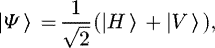 (1)
where |V〉 stands for a photon in a vertically polarized quantum state and similarly |H〉 stands for a photon in a horizontally polarized quantum state. Thus, the whole state vector of the system, |Ψ〉, is a quantum superposition of both the horizontal and vertical polarizations, this is known as a Q-bit state.1
(1)
where |V〉 stands for a photon in a vertically polarized quantum state and similarly |H〉 stands for a photon in a horizontally polarized quantum state. Thus, the whole state vector of the system, |Ψ〉, is a quantum superposition of both the horizontal and vertical polarizations, this is known as a Q-bit state.1
Once the state in equation (1) is obtained, the photon passes through a polarizing beamsplitter (PBS). By quantum theory we know that after passing through the PBS the state of the system, either |V〉 or |H〉, is an eigenstate of the polarization operator. The probability of obtaining each of them is given by the inner product with the initial state:
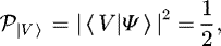
The PBS sends the photons that are projected onto |V〉 through one path and the ones are projected onto |H〉 through the other. This means that each photon can only take one of the two paths and can be detected by only one detector. Hence, we label the detectors 0 and 1. As the path taken by each photon is a quantum process with probability 50%, each detection is completely random. Therefore, the binary sequence generated via this process will be a random one.
2.1 Experimental setup
Since the interval of wavelengths at which the PBS works best corresponds to the red part of the electromagnetic spectrum, we take a 770 nm LED and pass its beam through a vertical polarizer. Then we use a convex lens to collimate the beam. Finally, the beam is lead through a half-wave plate that prepares the photons in the state given by equation (1), which then goes through the PBS.
To ensure that the state of the photons after going through the half-wave plate is actually the one described by equation (1), we calibrate it so that the proportion of arrivals in the two detectors is roughly 50–50. At the outputs of the beamsplitter, we place fiber couplers that are connected to single photon detectors. Figure 1 shows the setup implemented in the quantum optics laboratory.
It is possible that both detectors register a 1 and a 0 simultaneously. Nonetheless, this has to do with the time resolution of the detectors, rather than with the quantum physics associated with the process. Since each detector has a time interval during which it must process the pulse, if during the same interval another photon arrives at the second detector, both will send a signal, which will be registered as a simultaneous detection. In such a case, the corresponding entry in the random sequence must be discarded. In the Alternative experiment section we discuss another setup which would solve this issue.
 |
Fig. 1 Schematic diagram of the experimental setup. |
2.2 Statistical testing
The question of deciding if a sequence is random does not have a definite answer since the randomness criteria will vary between different applications. However, some unbiased statistical tests must be applied to a sequence in order to decide if it is sufficiently random for the purpose it is intended. It is important to recall that statistical testing only improves our confidence in the hypotheses that a given sequence randomness is acceptable, but will never prove it definitely [3].
A random sequence could be interpreted as the result of flipping an unbiased coin with sides labeled “0” and “1”, with independent flips having complete forward and backward unpredictability and equal probability. For the purpose of the statistical testing of our sequence and to have a quantitative measure of the randomness, we can formulate several statistical tests to assess the veracity of a given null-hypothesis. In this letter, we will define the null-hypothesis to be tested as the sequence being tested is random. Ideally one would like to apply a series of varied tests to the sequence in order to ensure a greater confidence in its randomness. Each test applied to the sequence gives a decision rule whether to accept or reject the null-hypothesis, and with each test the sequence passes the confidence in the hypothesis becomes stronger.
2.3 P-values and testing
The statistical tests in The NIST test suite [4] are designed to test the null-hypothesis The sequence is random, in contrast to the alternative hypothesis The sequence is not random. For each test a statistic2 is chosen, and the probability distribution is computed under the assumption of the null-hypothesis. Then a critical value is fixed, meaning we reject the null-hypothesis if the statistic exceeds such a value. For the NIST test, the critical value is set when the cumulative probability of the statistic reaches 99%.
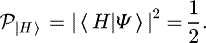
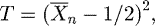
For example, a simple test to check if the sequence of ones and zeros is unbiased can be described as follows. We define the statistic:
 (2)
where
(2)
where  is the sample average. We should reject the null-hypothesis (E [Xi] = 1/2) if the value of the statistic is much greater than 0. The exact critical value c for which we reject the null-hypothesis if T > c is quite a delicate point. To define it, we fix a level of significance α0 and pick c such that
  (note that for a well-behaved statistic, such as T in this example, the value of c is completely determined by α0), where such a probability is to be computed under the assumption of the null-hypothesis . Intuitively speaking
  is the probability of rejecting the null-hypothesis given it is true, so we would want to choose α0 to be a small number close to 0.3
The above discussion gives a general idea of how one can construct statistical tests, but it is important to note that the number α0 is selected arbitrarily. Hence, we define the p-value as the minimum level of significance for which we will reject the null-hypothesis. The p-value is a relevant quantity since it makes no use of an arbitrarily chosen level of significance. Intuitively speaking the p-value is the probability of obtaining the value of the statistic we got or worse.
So, for instance in our example, if we have a sequence  , we can compute the value of the statistic
  and figure out the p-value just by computing the probability of the tail of the distribution
  . Note this is precisely the smallest level of significance for which we would have rejected the null-hypothesis, because if we would have picked a level of significance α0 > p we would have:
 (3)
and we would have rejected the null-hypothesis because t would be bigger than our threshold value c. On the other hand, if we would have picked a level of significance α0 < p we would have:
(3)
and we would have rejected the null-hypothesis because t would be bigger than our threshold value c. On the other hand, if we would have picked a level of significance α0 < p we would have:
 (4)
(4)
And we would have accepted the null-hypothesis as t would be smaller than our threshold value c (see Fig. 2 for a graphical aid). Hence for any level of significance less than p we would accept the null hypothesis and for any level of significance greater than p we would reject the null hypothesis, therefore p is the smallest level of significance for which we would reject the null-hypothesis. This construction gives us much more information, as for any given level of significance α0 we just compare it with the p-value. If the latter is smaller than the former we reject the null-hypothesis. Otherwise, we accept it.
Most of the tests used have more complicated statistics but the basic idea is the same: the p-value is the smallest level of significance for which we would reject the randomness hypothesis.
As we used plenty of tests, we have many p-values to interpret. The easiest way to do so is to check if the p-values are uniformly distributed. The plots in the Results section compress all that information into a single graph that is related to a test for which the null-hypothesis is: the p-values have uniform distribution.
 |
Fig. 2 In the plots above we see the density plot for the statistic T. As detailed in the main text we have performed an experiment for which the statistic T has value t (which can be seen in the plot), then the p-value for such a test is the green area (the area after t). Now at the left side, we see an example where we have chosen a level of significance (the area of the blue region, which is the area after c) greater than p, hence t is greater than our threshold value c. On the right we see an example where we have chosen a level of significance less than p, hence the value t is less than our threshold value c. Note that in some regions the two colors overlap. |
2.4 NIST Statistical test suite
Throughout this work, we used the National Institute of Standards and Technology statistical test suite for random number generators [4], which is a suite composed of 15 tests designed to assess the randomness of long binary sequences produced either by true random number generators or pseudo-random number generators. This suite was chosen due to its practicality in dealing with binary sequences produced in our setup, the stringency of its tests, its wide documentation and since it is an industry standard in random number testing.
The NIST Statistical test suite is designed to test the randomness of binary sequences of lengths between 103 and 107 bits. Among the various tests there are:
-
Frequency tests: check that the proportion between ones and zeros is roughly 1/2.
-
Runs tests: look at the length of subsequences of only one kind of bit.
-
Cumulative sums tests: check for too many zeros or ones either at an early or late stage in the sequence.
-
Matrix rank test: check that the ranks of matrices, whose columns are vectors from the sequence, have the expected behavior. For more detailed information, see [5].
-
Fourier transform tests: that check for repeating patterns.
-
Overlapping tests: verify that the occurrence of subsequences of different sizes are as expected and are separated from each other as expected in a truly random sequence.
-
Random excursion tests: check that, if a random walker chooses direction according to the bits in the sequence, it moves as expected.4
-
Approximate entropy tests: check the non-uniformity in the joint distribution for m-length subsequences.
-
Linear complexity tests: check for the length of a linear feedback shift register for sequential dependence. The purpose of this test is to assess the complexity of the sequence. Random sequences are characterized by a longer feedback register, and a short feedback register implies non-randomness. For details, see [4,6].
All of these tests are run in both the whole sequence and in blocks made up of subdivisions of the original sequence. The length of the subdivided sequence is constant and is entered as an input to the program. Consequently, both the versatility of the suite and the stringency of the tests it contains, make it a complete and reliable tool for the assessment of the randomness of our data. As a last and fairly important remark, one may note that this set of tests is designed for perfect coin toss-like experiments, where the chances are 50–50; hence, data exhibiting a large bias will have a high probability of failure in most tests [4]. Due to technical and experimental handicaps, our generator was not perfect coin toss-like, having a slight yet noticeable bias that required a postprocessing of the data with a simple algorithm before the application of the test suite. The origin of the bias had to do with the alignment of the equipment (the wave-plate and the beamsplitter) and with the physical defects they had from the manufacturer. It should be expected that with higher quality optical components, as with better alignment, the bias in the data would be reduced.
2.5 von Neumann’s bias removal
As noted before, due to imperfections in the setup, some bias is to be expected in our final data. Since the usual tests for randomness of binary sequences are designed for unbiased random variables [4], we may apply von Neumann’s algorithm [7] to produce a shorter unbiased sequence from our original experimental sequence.
Von Neumann’s algorithm is a straightforward procedure consisting in dividing the data into pairs, and replacing each pair using the following rule: if the pair is either 00 or 11 it is removed from the sequence. If the pair is 10 it is replaced by a 1 and if the pair is 01 it is replaced by a 0. Even though this algorithm reduces the length of the sequence to less than a quarter, it has the advantage that we don’t need to know the bias of the initial sequence and the output sequence is an unbiased one. Thus, under the assumption that each bit in the original sequence is independent of the others we can produce an unbiased sequence.
To prove that the sequence obtained after the described procedure is unbiased and independent, consider a set of random variables (in our case polarization measurements) M1, M2, … , MN such that the probability of getting a 1 is  and the probability of getting a 0 is
  . Then, as each measurement is independent:


Hence both combinations, 10 and 01, are equiprobable and the algorithm delivers an unbiased sequence. Since the original variables are independent, every function of say the first and second variables is independent of every other function of say the third and fourth variables, consequently independence is conserved. Therefore we can conclude that von Neumann’s technique should remove the bias of the sequence without destroying its independence.
Some refinements to von Neumann’s technique and some new techniques to generate an unbiased random sequence are described by Elias [8] and Peres [9], but due to its straightforward character, simplicity and the amount of data obtained we choose to use von Neumann’s algorithm, despite the shortcoming of reducing considerably the length of the sequence.
2.6 Quantile–quantile plots
Quantile–quantile plots are a great visual tool to check if a sequence follows a given a distribution. The basic idea of this method is as follows. Given a sample  of size N, which we think has a given distribution, we would expect that for a given x the number of values in
  divided by N (the amount of data) is close to cumulative distribution function (F) evaluated at x.
 (5)
the function at the right is called the empirical distribution function:
(5)
the function at the right is called the empirical distribution function:
 (6)
(6)
And we are naturally interested in comparing F and Femp, and the usual way to do it is to plot the set of points  . If the sequence
  indeed follows such distribution the points should all lie on a straight line of slope one.
These plots will be used in assessing if the distribution of p-values is uniform over the interval [0, 1] as expected [10].
3 Results
With the previously addressed setup, a total of two hours of data was collected. After the pooling was completed, a total of 13 837 005 single photon arrivals were recorded in both detectors such that the measured bitrate was approximately 1.9 kb/s.
3.1 Biased sequence
With these roughly 1.4 × 107 bits, we made sequences of ones and zeros of length 1 × 10⁵ and applied the NIST Statistical tests to different partitions of the sequence. This particular length of the smaller subsequences is recommended for maximum reliability and efficiency in the documentation of the test suite [4]. Due to the amount of bits that were assessed, some tests were repeated more than once. In total, 188 tests were applied to all the sequences. Each test resulted in a corresponding p-value as was previously mentioned.
From the 188 test conducted, the sequence failed 21 of them as shown in Figure 4(a), which is far from the 2 expected that can be accounted due to statistical fluctuations.5 Also, as previously mentioned, a requirement for our sequence to be considered random is not only for it to pass the several statistical tests, but that the p-values follow a uniform distribution. However, the quantile–quantile plot in Figure 3 shows that the distribution of p-values is not uniform due to the bias. Since the quantile–quantile plot of a cumulative uniform distribution is a straight line with slope 1, we expect that after applying von Neumann’s algorithm to our sequence, the quantile–quantile plot of p-values should resemble a straight line.
 |
Fig. 3 Quantile–quantile plot of the empirical cumulative distribution (dotted) vs. the cumulative distribution of a uniform random variable (solid line). We can see that there is a clear deviation of the data from the straight line before applying the bias removal algorithm. |
3.2 Unbiased sequence
After applying von Neumann’s algorithm in order to remove the bias, the 1.4 × 107 bits long sequence was reduced to a length of 3 400 052 bits. We applied to this unbiased sequence the various statistical tests in the NIST suite. A sample of the results and the corresponding p-values obtained are shown in Table 1. The proportion column in Table 1 refers to the fraction of the 34 bit-streams of 105 bits6 that passed the test.
The distribution of p-values is shown in Figure 4. As it can be seen the sequence failed two out of the 188 tests, around the expected value of 1.8. In the plot of Figure 5 we see a major improvement in the distribution of p-values, meaning the bias correction algorithm improved significantly the uniformity of p-values in the NIST tests.
We also proceed to test the uniformity of the p-values. In the plot in Figure 5 we see a quantile–quantile plot of the empirical cumulative distribution function of the p-values vs. the distribution function of a uniform random variable. The resemblance is easily seen and the p-values look like that they have a uniform distribution.
To prove this more formally we made a Kolmogorov–Smirnov test to test the null-hypothesis: The p-values follow a uniform distribution. Details can be found in [10]. The p-value obtained in that test was p = 0.8211.
To compare this result, the p-value for the same test with the biased sequence was 2.49 × 10⁻⁸. So the uniformity hypothesis of the p-values for the biased sequence will be rejected for our level of significance of 0.01, while the uniformity hypothesis of the p-values for the unbiased sequence will be accepted.
Partial results of the NIST suite for our unbiased binary sequence.
4 Discussion
We compare our results with previous attempts at this setup. These attempts have achieved up to 2 × 109 bits in a pooling time of thirty minutes and with an average intensity of 5 × 10⁵ photons per second [12]. This means that previous settings were able to produce a bitrate greater by roughly three orders of magnitude. The discrepancy is attributed to the difference in the LED intensity between both setups. Furthermore, in [12], more intensity ranges were studied and it was concluded that higher intensity not only improves the bitrate but also the performance in the NIST test suite.
However, it is to be noted that this is a very good in comparison to the highest bitrate designs that are in use today, of roughly 4 Mb/s [13]. Therefore, our bitrate in addition to both the low cost and low complexity of our setup make our implementation of the quantum number generator a great alternative option for the standard user seeking a fairly large sample of binary digits for simple cryptographic or simulation purposes.
4.1 Comparison to other random number generators
In this section, we compare our random number generator implementation to both radioactive decay random number generators and pseudo-random number generators.
First, pseudo-random numbers were generated using the rand( ) function of the C programming language. To assure comparability we generated the same number of bits as the ones that were left after the von Neumann algorithm. The results of the test suite are shown in Figures 4 and 6. Notice the deviation from the uniform distribution in the quantile–quantile plot for the pseudo-random generator.
To compare with true random numbers generated by timing successive pairs of radioactive decays detected by a Geiger-Müller tube interfaced to a computer, we resorted to the use of Hotbits [11]. At Hotbits we can access both sequences of random digits and NIST test results being applied to random sequences obtained by tracking radioactive decays. The results from applying the NIST test suite are shown in Figures 4 and 7. As it is easily seen in Figures 5 and 7 the most uniformly distributed p-values correspond to both our sequence after the application of von Neumann’s algorithm and the bits obtained from Hotbits, which is an indication that our setup is indeed a very good implementation of a random number generator.
The most notorious thing that could be improved for future implementations is the bitrate of our setup. The main problem with the bitrate compared to other implementations [12] was that the intensity of the LED we used was not optimal. Furthermore, by applying von Neumann’s algorithm the sequence is further reduced in length, diminishing the bitrate. But in general, we can achieve both uniformity and higher bit rate by increasing the intensity of the LED. Nevertheless, the maximum bitrate is bounded by the capacity of the detectors to withstand high-intensity light. This problem was not considered in the present work but can be addressed for future implementations.
 |
Fig. 4 Scatter plot of the p-value results for 188 tests performed on binary sequences that were generated by various methods, the red line denotes the threshold for which the p-value indicates that the sequence has not passed a given test. (a) The sequence generated using LED light passing through a polarizing beamsplitter. (b) Same sequence after applying the von Neumann’s algorithm for bias removal. (c) Pseudo-random numbers generated with the rand( ) method in the C programming language. (d) Random numbers taken from the true random number generator implemented by Hotbits [11]. We can see how von Neumann’s algorithm greatly improves the performance of our random number generator. |
 |
Fig. 5 Quantile–quantile plot of the empirical distribution of p-values (dotted) vs. a uniform distribution (solid lines) of our data after applying von Neumann’s bias removal algorithm. |
 |
Fig. 6 Quantile–quantile plot of the empirical distribution of p-values (dotted) vs. a uniform distribution (solid line) for rand( ) pseudorandom number generator from C programming language. |
 |
Fig. 7 Quantile–quantile plot of the empirical distribution of p-values (dotted) vs. a uniform distribution (solid line) for Random bits from Hotbits [11]. |
5 Dead-end
An important part of the data gathering is the proper alignment of the optical elements in the setup, in particular, the half-wave plate and the PBS. Since we used fiber couplers for each detector, the alignment of the beam and the optical fiber is crucial in order to acquire meaningful data. Thus, the alignment process required a lot of time and effort. Nevertheless, the collected data presented a noticeable bias due to inaccuracies in the alignment of the setup. At first the origin of the bias was not clear to us and consequently, the statistical test results were not meaningful to assess our generator as being or not being random. However, after realizing the existence of a bias in the data we applied von Neumann’s algorithm to correct it and obtain meaningful results from the NIST test suite.
Another difficulty we faced was at the data analysis stage. The software available in the quantum optics laboratory for data acquisition delivered a huge set of files in a non-conventional format that was very difficult to convert into a compact and useful data set. In order to apply the NIST tests we had to decode and convert the original data file into a .txt file that was used as an entry parameter for C program used in the NIST suite.
6 Alternative experiment
It is worth mentioning an alternative setup that solves the problem of the simultaneous detections. This problem arises because even if we filter the beam that comes from the LED, it could happen that the photons arrive at the detectors at a larger rate than the detectors are able to differentiate. The setup that optimizes this issue is based on a single photon source (Fig. 8).
The single photon source uses a process known as Spontaneous Parametric Down Conversion (SPDC). This process consists of making a laser beam pass through a non-linear crystal, which absorbs the incoming photon and emits an entangled pair. Therefore, one of the resulting photons serves as a signal (in detector D3) whereas the other photon enters our setup. Thus, the time correlation between 1’s and 0’s is significantly improved.
Even when we can make all the data valid within this procedure, the rate of the single photon source of our laboratory is not as high as the rate of photons that arrive at the detectors when the setup with the LED as a source is implemented. Due to availability in the quantum optics laboratory, we used a LED as the source of light but perhaps, if we had implemented a laser instead, the bitrate would have been higher.
 |
Fig. 8 Schematic diagram of the alternative setup. |
7 Conclusions
In this letter, a simple method for generating random numbers in the quantum optics laboratory was described and the results of this implementation were analyzed. The method consists of preparing photons emitted by a LED in a superposition of vertical and horizontal polarization states. After that, a polarizing beamsplitter is used to generate a random number sequence depending on the path taken by the photons. After processing the data, the NIST test suite for the validation of random number generators was applied to the processed sequence and the results were analyzed and compared with other random and pseudo-random number generators. This allowed us to conclude that the setup developed is an appropriate implementation of a quantum random number generator.
Additionally, we discussed an alternative experimental setup based on SPDC which solves the time correlation problems that our random generator exhibits. As well as several ways of optimizing the bitrate. We conclude that it is more efficient to consider the proposed setup and drop some data than the alternative SPDC based implementation. Finally, the experiment we performed is much easier to implement than the one with the single photon source. If one were to produce a commercial device that generates truly quantum numbers, the second proposal would be very unpractical.
Acknowledgments
The authors would like to thank the Physics department of Universidad de los Andes for their support at the IPT 2016. We would like to especially thank professors Alonso Botero and Juan Manuel Pedraza for their guidance and preparation for the tournament. In addition, we would like to thank professor Alejandra Valencia and all the staff at the quantum optics laboratory at Universidad de los Andes for all the help and advice in working the details and implementation of the quantum number generator.
Appendices
Appendix
Here we present the characteristics of the setup and of its optical components:
-
height: 11.700 ± 0.001 cm;
-
distance between the PBS and the fiber couplers: 6.420 ± 0.001 cm;
-
focal distance: 3.50 ± 0.01 cm.
See Table 2.
Description of the optical components used in the setup.
References
- W. Diffie, M.E. Hellman, Privacy and authentication: an introduction to cryptography, Proc. IEEE 67, 397 (1979) [CrossRef] [Google Scholar]
- G.B. Agnew, Random sources for cryptographic systems (Springer, Berlin, Heidelberg, 1988), pp. 77–81 [Google Scholar]
- D.E. Knuth, The art of computer programming (Addison-Wesley Pub (Sd), Reading, MA, 1981), Vol. 2, 2nd ed. [Google Scholar]
- NIST, Statistical test suite (2014), http://csrc.nist.gov/groups/ST/toolkit/rng/documentation_software.html [Google Scholar]
- I.N. Kovalenko, Durri-Hamdani, Distribution of the linear rank of a random matrix, Theor. Prob. Appl. 17, 342 (1972) [CrossRef] [Google Scholar]
- A. Klein, Linear feedback shift registers (Springer, London, 2013), pp. 17–58 [Google Scholar]
- J. von Neumann, Various techniques used in connection with random digits, J. Res. Nat. Bur. Stand. 12, 36 (1951) [Google Scholar]
- P. Elias, The efficient construction of an unbiased random sequence, Ann. Math. Statist. 43, 865 (1972) [CrossRef] [Google Scholar]
- Y. Peres, Iterating von Neumann’s procedure for extracting random bits, Ann. Statist. 20, 590 (1992) [CrossRef] [Google Scholar]
- M.H. DeGroot, M.J. Schervish, Probability and statistics. Addison-Wesley series in statistics (Addison-Wesley, Boston, MA, 2002) [Google Scholar]
- J. Walker, Hotbits (1996), www.fourmilab.ch/hotbits/ [Google Scholar]
- N. Barbosa, Quantum random number generators using photons, Undergraduate thesis, Universidad de los Andes, 2013, pp. 28–34 [Google Scholar]
- IDQ, Random number generation using quantum physics (2010), http://www.idquantique.com/wordpress/wp-content/uploads/quantis-whitepaper.pdf [Google Scholar]
A Q-bit is a two-level quantum system, and a Q-bit state is a state of such a system.
Function that assigns a number to each sequence.
In our case we pick α0 = 0.01.
A random walk in this case is a sequence of steps in one dimension starting at the origin, corresponding to a unit step to the left (a zero) and to a unit step to the right (a one).
0.01 × 188 = 1.8 ≈ 2, level of significance times the number of tests.
This number is an input parameter in the NIST software having to do with the desired sample size to be tested.
Cite this article as: Santiago Aguirre, Juan Diego Arango-Montoya, David Jaramillo-Duque, Juan Felipe Méndez, Nicolás Morales-Durán, Mateo Restrepo, A quantum random number generator implementation with polarized photons, Emergent Scientist 1, 2 (2017)
All Tables
All Figures
|
Fig. 1 Schematic diagram of the experimental setup. |
| In the text | |
|
Fig. 2 In the plots above we see the density plot for the statistic T. As detailed in the main text we have performed an experiment for which the statistic T has value t (which can be seen in the plot), then the p-value for such a test is the green area (the area after t). Now at the left side, we see an example where we have chosen a level of significance (the area of the blue region, which is the area after c) greater than p, hence t is greater than our threshold value c. On the right we see an example where we have chosen a level of significance less than p, hence the value t is less than our threshold value c. Note that in some regions the two colors overlap. |
| In the text | |
|
Fig. 3 Quantile–quantile plot of the empirical cumulative distribution (dotted) vs. the cumulative distribution of a uniform random variable (solid line). We can see that there is a clear deviation of the data from the straight line before applying the bias removal algorithm. |
| In the text | |
|
Fig. 4 Scatter plot of the p-value results for 188 tests performed on binary sequences that were generated by various methods, the red line denotes the threshold for which the p-value indicates that the sequence has not passed a given test. (a) The sequence generated using LED light passing through a polarizing beamsplitter. (b) Same sequence after applying the von Neumann’s algorithm for bias removal. (c) Pseudo-random numbers generated with the rand( ) method in the C programming language. (d) Random numbers taken from the true random number generator implemented by Hotbits [11]. We can see how von Neumann’s algorithm greatly improves the performance of our random number generator. |
| In the text | |
|
Fig. 5 Quantile–quantile plot of the empirical distribution of p-values (dotted) vs. a uniform distribution (solid lines) of our data after applying von Neumann’s bias removal algorithm. |
| In the text | |
|
Fig. 6 Quantile–quantile plot of the empirical distribution of p-values (dotted) vs. a uniform distribution (solid line) for rand( ) pseudorandom number generator from C programming language. |
| In the text | |
|
Fig. 7 Quantile–quantile plot of the empirical distribution of p-values (dotted) vs. a uniform distribution (solid line) for Random bits from Hotbits [11]. |
| In the text | |
|
Fig. 8 Schematic diagram of the alternative setup. |
| In the text | |
Current usage metrics show cumulative count of Article Views (full-text article views including HTML views, PDF and ePub downloads, according to the available data) and Abstracts Views on Vision4Press platform.
Data correspond to usage on the plateform after 2015. The current usage metrics is available 48-96 hours after online publication and is updated daily on week days.
Initial download of the metrics may take a while.