| Issue |
Emergent Scientist
Volume 3, 2019
|
|
|---|---|---|
| Article Number | 1 | |
| Number of page(s) | 8 | |
| Section | Physics | |
| DOI | https://doi.org/10.1051/emsci/2018006 | |
| Published online | 01 February 2019 | |
Research Article
Cross-camera tracking and frequency analysis of a cheap Slinky Wilberforce pendulum
Grenoble INP − PHELMA,
Grenoble,
France
* e-mail: This email address is being protected from spambots. You need JavaScript enabled to view it.
Received:
10
April
2018
Accepted:
11
December
2018
Abstract
A Wilberforce pendulum is a mechanical oscillator often used as an example for the effect of coupling. After establishing a theoretical model of this oscillator and building a prototype, tracking algorithms have been developed to get the position of the oscillator. These tools enable us to highlight the existence of normal modes and determine the constants of the system. We also test different initial conditions to project the state of the pendulum on the normal modes. At the end, we discuss the match between our model and the experimental results. This comparison leads to possible improvements of the model and of the measurements.
Key words: Wilberforce pendulum / classical mechanics / position measurements / video tracking / frequency analysis
© P. Devaux et al., Published by EDP Sciences, 2019
 This is an Open Access article distributed under the terms of the Creative Commons Attribution License (http://creativecommons.org/licenses/by/4.0), which permits unrestricted use, distribution, and reproduction in any medium, provided the original work is properly cited.
1 Introduction
The Wilberforce pendulum has been named after the British physicist L.R. Wilberforce, who invented and studied this pendulum at the end of the 19th century [1]. It is a coupled mechanical oscillator composed of a mass suspended to a spring and free to turn around the vertical axis of the system. A sketch of the system is shown in Figure 1. At first sight, the motion of the pendulum seems to be disordered. However, with a closer look, we notice that the pendulum has two motions, the translation and the rotation, whose intensities are linked: when one is very strong, the other is almost nonexistent. Thus, although relatively basic and without industrial applications nowadays, this pendulum is an excellent example to grasp the principle of coupling.
In 1894, Wilberforce established the first theoretical study with experimental assessment of the movement of the pendulum [1]. However, our work is more based on the studies carried on by Berg and Marshall, who pointed out and studied the eigenmodes of the system, but without detailing how to measure their frequencies [2]. We were also inspired by Mewes in the building of our cheap prototype, as he used a Slinky spring in its general presentation of the oscillator [3]. There are different possible experimental setups that have already been explored to study the motion of a Wilberforce pendulum. A common way to measure the vertical displacement for instance is based on an ultrasonic distance sensor [4], possibly used together with a camera [5].
We present here the development of a convenient toolbox named Measurements of Oscillations by Video Extraction (MOVE) within the framework of our first year physics project at PHELMA [6]. Since our project was strongly time- and cost-limited, it has been decided to focus on cross-camera tracking for the measurement of both vertical and angular displacements. Based on MATLAB algorithms to detect and process the movement, MOVE enables us to perform a frequency analysis which highlights two eigenmodes and determines their frequencies. By comparing our theoretical model and experimental results, possible improvements can be identified for the model and for measurement methods.
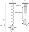 |
Fig. 1 A sketch of our prototype of the Wilberforce pendulum at its equilibrium state (a) and in motion (b). |
2 Methods
2.1 Theoretical model
The first hypothesis of this model is the introduction of a potential energy E
pot of coupling between linear and rotational movements [2,3]. The shape of this coupling potential has been admitted considering what had already been used in the literature. When the pendulum is rotated by an angle θ and elongated by a length z compared to its equilibrium state, E
pot writes:
 (1)
(1)
where ϵ is called the coupling constant, of about 10−2 N rad−1.
Then, we set the equations of motion up by using Newton's second law of motion and the angular momentum theorem (along the z axis): (2)
(2)
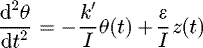 (3)
(3)
Here, k and k ′ are respectively the spring constant (N m−1) and the torsion constant (N m rad−1). m and I are the mass (kg) and moment of inertia (kg m2) of the pendulum (both being easily adjustable in our prototype).
Those coupled equations can be solved using Laplace transform. By imposing particular initial conditions (i.e. a vertical and/or an angular displacement from the equilibrium, respectively, called z
0 and θ
0, but no vertical or angular speed when the motion begins), the previous system becomes, in Laplace space: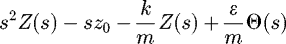 (4)
(4)
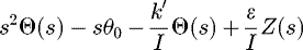 (5)
(5)
This polynomial system can be solved, and we obtain: (6)
(6)
with (7)
(7)
 (8)
(8)
 (9)
(9)
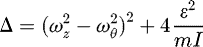 (10)
(10)
We will suppose that the two frequencies of our system match [2,3], i.e.  (11)
(11)
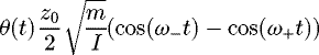
This assumption corresponds to the condition of resonance [7]. It is made acceptable by a careful adjustment of our pendulum's moment of inertia. It allows us to highly simplify the expression of z(t) and θ(t):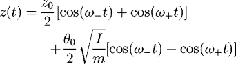 (12)
(12)
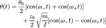 (13)
(13)
and the frequencies are also simplified: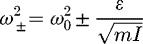 (14)
(14)
Thus, the main objective of this work is to build our own prototype, and get data about the evolution of both altitude and deviation angle with time. Those data can then be compared to the model to see its limits.
2.2 Experimental setup
The lower part of the pendulum is a metallic empty can. It is pierced four times in such a way that we can cross the two threaded rods with a 90° angle in the middle of the can (Fig. 2). The positions of these threaded rods are fixed thanks to nuts in the external surface of the can. In addition to that, some extra nuts have been used in order to adjust the moment of inertia, and stabilize the system, which is crucial to observe the phenomenon. Indeed, it may be necessary to modify the inertia of the system without changing its mass, and this can be done by moving the nuts along the rods. All the dimensions and characteristics are indicated in Table 1.
The other important part of the pendulum is the spring. It has to be flexible enough to be easily elongated, which means that the spring constant must be weak (in the range of a few N m−1). Moreover, the spring should be allowed to turn on itself when it is vertically stretched so that the phenomenon can be observed. An appropriate spring is a “Slinky” spring [3] (see its dimensions in Tab. 1), and it is precisely this kind of spring that has been used for our prototype. One of its ends is fixed to an immobile stand above the can, while the other end is fixed to the can with the help of four cable ties. The spring has been shortened by tieing some of its upper coils to fit with the height of our experimental room.
Designed this way, our coupled system has both linear and rotational modes, switching from one to the other. As it moves freely, it will periodically switch between pure translation and pure rotation through a mix of both movements known as the “Wilberforce effect”.
We fixed the free end of the Slinky at 3.75 m above the ground. At equilibrium, the bottom of our prototype was 1.20 m above the ground. To record the movement of the pendulum, we used video capture, which offers the advantage to be cheap and flexible without needing any specific material. The system has been marked with three black areas. A large black strip has been fixed around the cylindrical part (see Fig. 2) and two black dots with different sizes have been drawn on the lower face of the can. One of the dots is placed at the centre of the face and the other one close to its edge.
The experiment consists in shooting the motion along two perpendicular directions with two cameras at the same time (see Fig. 3). One shoots the vertical movement of the system from the side and the other from below, targeting the bottom of the can. It is also necessary to pay attention to the lighting of the experiment. We add an extra light source on the ground to get a more luminous image of the bottom of the can.
Dimensions and masses of all pendulum components. Note that the length of the spring was measured when it was fully compressed.
 |
Fig. 2 Views of our hand-built prototype. |
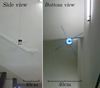 |
Fig. 3 Snapshots of the pendulum as captured by the two cameras. |
2.3 Development of the MOVE toolbox
The basic idea is to detect the targets put on the can by contrast with the rest of the image. For its convenience and with a view to process each image as a matrix, we have chosen MATLAB as our main developing tool. Positions of the pendulum are extracted from mp4 videos, either with 480 × 320 or 640 × 480 resolution and acquired at the rate of 30 fps.
Each movement has its own processing because we have to extract different physical quantities with different issues. The video in color is treated as a four-dimensional array which is transformed into a three-dimensional array to consider only images in shades of gray. Each frame of the movement is a two-dimensional array.
The MOVE algorithm dedicated to linear movement is based on the comparison between the frame processed and an associated background [8]. The background is a dilation of the frame calculated with five images. This is comparable to an opening time of 1/6 s (167 ms) in photography. The comparison consists in an absolute difference between the frame and the background. This way, every pixel of the image that did not change is set to zero, which is equivalent to black color. We obtain an image composed massively of black pixels and few gray and white pixels that match with moving areas between two frames. To isolate the relevant object to track, we proceed to a threshold calculation by the Otsu method [9]. Every pixel which has a value higher, or equal, to the calculated threshold has its color code set to 255 (white). The other pixels are set to 0 (black). We finally have a binary image of the object from which we can extract the coordinates of the biggest area, supposed to be the can. The vertical coordinates can be printed directly for each frame to get linear position versus time. Yet, results appear to be noised, which makes reconstruction from the last evaluated position necessary. For this purpose, a box is centred on the first evaluated value of the altitude. In this box, only the darkest pixels are selected according to an imposed threshold. The result consists in a binary image with few areas of different sizes. The biggest area is expected to match with the black strip fixed around the can. By printing the vertical position of this object for each frame, a better estimation of the linear displacement is finally obtained.
The MOVE algorithm dedicated to rotational movement works directly with the detection of black dots under the can. To detect only those dots, it is essential to limit the scanned area to the disk at the bottom of the can containing the dots.
A mask is created for each frame to select only the pixels inside the scanned disk. Within this area, a threshold is calculated and dots are selected accordingly, in the same way as for linear movement. It is necessary to keep only the two biggest objects (as the best candidates for the two black dots) and save the coordinates of their centres (see Fig. 4).
Measuring the angle between the line passing through the dots and a reference horizontal line is not direct. Polar transformation easily gives such an angle, but included in [ − π, + π]. A post-processing step based on its previous values is necessary to rebuild a continuous curve, as shown in Figure 5.
 |
Fig. 4 Comparison of a raw (a) and a processed frame (b) extracted from a rotational movement. |
 |
Fig. 5 Comparison between the geometrical angle in [ − π, + π] and the post processed angle, corresponding to our final values of θ versus time. |
3 Results
3.1 Typical results
To observe the Wilberforce effect, a simple vertical displacement of the pendulum is initially needed. So, θ0 = 0 is the initial condition to be applied in this case. Thus, the equations of the motion become: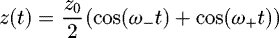 (15)
(15)
 (16)
(16)
The most obvious behaviour that can be observed when looking at the obtained Wilberforce effect (Fig. 6) is the energy switch between the linear and the rotational motions. When the amplitude of translation is at one of its peaks, the pendulum does not spin a lot, and vice-versa. This can be easily explained by the total energy of the system depending on both z and θ: its conservation prevents the two motions to reach their peaks at the same time.
Additionally, the theoretical model forecasts that the motions of the pendulum are linked to periodic functions. However, this is hardly noticeable in Figure 6. In order to remove any doubt, further analysis of these curves is mandatory.
 |
Fig. 6 Results of the main experiment, highlighting the “Wilberforce effect” behaviour. |
3.2 Frequency analysis of the Wilberforce effect
According to (15) and (16), the movement of the Wilberforce pendulum is made of the two frequencies ω + and ω − which can be revealed by spectral analysis. The MATLAB fast Fourier transform (FFT) algorithm proposed by MATLAB [10] has been used for that purpose, and the result is displayed in Figure 7.
This figure proves that translation and rotation oscillate as predicted with almost the same frequencies. Those frequencies are written down in Table 2. They are calculated for each motion (translation and rotation), and the measurement uncertainty is due to the accuracy on the discrete frequencies. We can then combine these two results in order to obtain more precise values [11].
The pendulum movement is thus a superposition of two simpler periodic motions, each one composed of only one frequency: these are the normal modes of the Wilberforce pendulum.
Given that z and θ seem to have similar behaviours, we will only focus on z(t) in what follows.
 |
Fig. 7 Spectral analysis of the Wilberforce effect, performed with MATLAB FFT. |
Values of ω − and ω + obtained with the spectral analysis of the experimental curves.
3.3 Isolation of the two eigenmodes
Let us rewrite equation (12):
If we want the pendulum to oscillate at the ω + (resp. ω −) frequency, we have to cancel the term 
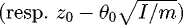 . This only depends on the initial conditions we choose to apply on our system. Letting the pendulum freely turn around its axis while displacing it vertically amounts to impose
  . Then z(t) and θ(t) will be in phase, oscillating at the ω− frequency in a so-called “symmetric mode”. On the contrary, if we turn the pendulum with the opposite angle −θ
0 while displacing it vertically, we will have
. Then z(t) and θ(t) will be in phase, oscillating at the ω− frequency in a so-called “symmetric mode”. On the contrary, if we turn the pendulum with the opposite angle −θ
0 while displacing it vertically, we will have  . Then z(t) and θ(t) will be in antiphase, oscillating at the ω
+ frequency in the “antisymmetric mode”.
. Then z(t) and θ(t) will be in antiphase, oscillating at the ω
+ frequency in the “antisymmetric mode”.
Hence, the initial conditions play an important role in the behaviour of the pendulum. Although we do not have a precise system to measure altitude and angle deviation, we are able to project the system on its symmetric mode because the initial conditions required match with the natural behaviour of the spring. However, the condition needed to observe a perfect antisymmetric mode is more difficult to realize experimentally, which explains that ω− appears in the spectrum of this mode (see Fig. 8).
 |
Fig. 8 Translation movement and associated spectral analysis of each normal mode. |
4 Discussion
4.1 Analysis of a few slight discrepancies
Analyzing the discrepancies between predicted and measured oscillations supposes to first evaluate as precisely as possible the values of all the constants.
The case of corrected constants m and I is special. The spring is quite heavy and it has an influence on the whole system behaviour. Thus, a correcting fraction of its mass m
s
has been added to the total mass of the pendulum, and the same to its moment of inertia I
s
. According to [12], this correction depends on the ratio  , where M is the mass suspended to the spring. Here,
  and we obtain m
corr = M + 0.348m
s
. Then, the spring constant k is obtained by measuring the vertical elongation of the spring when a load is added. ϵ and k
′ are deduced from frequencies of the system, given by spectral analysis. Indeed, (14) amounts to a system of two equations having k
′ and ϵ as unknowns (using ω
0 = ω
θ
).
and we obtain m
corr = M + 0.348m
s
. Then, the spring constant k is obtained by measuring the vertical elongation of the spring when a load is added. ϵ and k
′ are deduced from frequencies of the system, given by spectral analysis. Indeed, (14) amounts to a system of two equations having k
′ and ϵ as unknowns (using ω
0 = ω
θ
).
Now that all the constants of the system have been evaluated, the experimental results can be examined. The spectral analysis of the Wilberforce effect (Fig. 7) shows that, unlike our predictions, the amplitudes are not the same for the two frequencies (for both movements). Two possible reasons have been investigated. The first one is the inaccuracy of the initial conditions, i.e. θ0 is non-zero. However, the difference is too important to be only due to this slight error. A second, strongest approximation is the equality of the two frequencies ωz and ωθ in the model. Although the pendulum has been conceived to fit this condition, it was only on the basis of approximate values of k′, ϵ, m and I (as it has been discussed above).
Hence, the constants calculated in Table 3 are dependent on these approximations. To have an idea of the error we made, we can compare  and
and  which are supposed to be equal. With the constants in Table 3, we obtain: ω
z
= 2.18 ± 0.03 rad s−1 and ω
θ
= 2.49 ± 0.09 rad s−1, which shows that these two frequencies, supposed perfectly equal by our model, are in reality slightly different.
which are supposed to be equal. With the constants in Table 3, we obtain: ω
z
= 2.18 ± 0.03 rad s−1 and ω
θ
= 2.49 ± 0.09 rad s−1, which shows that these two frequencies, supposed perfectly equal by our model, are in reality slightly different.
To understand the source of errors which cause different amplitudes in the spectrum (Fig. 7), we can try to suppose θ
0 ≠ 0. For a vertical deviation of 60 cm we can suppose θ
0 = 0.5 rad as we know that we are very imprecise on the initial angle deviation. Thus, we can estimate the relative difference between the amplitudes obtained with FFT as  . From Figure 7, we obtain 33% of relative difference. Considering an initial angle different from zero is not sufficient to explain such big discrepancies between the amplitude of ω
− and ω
+. This is another argument to reconsider the hypothesis of resonance condition.
. From Figure 7, we obtain 33% of relative difference. Considering an initial angle different from zero is not sufficient to explain such big discrepancies between the amplitude of ω
− and ω
+. This is another argument to reconsider the hypothesis of resonance condition.
Corrected, measured and calculated constants of the system.
4.2 Adding friction to the model
We can see in Figure 6 that the pendulum is clearly underdamped. This is due to the effect of air friction, which was first neglected to simplify analytical solving.
As we have a coupled oscillator, the accurate effect is complex because there may be two damping coefficients, one for each type of motion. As a first attempt to quantify friction, we will only consider a simple exponential decrease of the linear amplitude and will assume that frequencies remain constant. Thus, (15) is now written: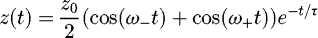 (17)
(17)
To extract the constant τ from the experimental data, we use an optimization function (based on the Nelder–Mead simplex algorithm) to minimize the residual sum of squares (RSS) between our model and the experimental points [13]. However, for the algorithm to return consistent results, it was necessary to suppress the major source of discrepancies due to the model (and independent from friction), which is the resonance hypothesis. Thus, we rather used a more general equation for the optimization algorithm, where the two cosines can have different amplitudes (which is the case when the condition of resonance is not verified):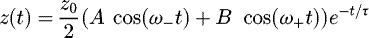 (18)
(18)
The results obtained this way are represented on Figure 9. As the model is more general, it fits well with the experimental data. But it is relevant to compare the agreement between this model and a model as general but without exponential decay, to evaluate the pertinence of this damping representation. The results of those two models are given in Table 4.
First, as one may expect, the values extracted for ω− and ω+ are close to the ones obtained through the spectral analysis (Tab. 2). The τ coefficient is also of the same order of magnitude than the one that can be extracted from the symmetric mode (53.3 s), given that we managed to obtain a pure underdamped sine wave for it (see Fig. 8). The hypothesis of modelling the effect of air friction by a mere exponential decay seems to be a reasonable assumption, given the values of the Pearsons R 2.
 |
Fig. 9 Experimental data and optimized fitting of z(t). |
Influence of the adding of an exponential decrease on the fitting of an experimental curve representing the pendulum motion along z. As the values in the table are algorithmically determined, no uncertainty is given here.
4.3 Possible improvements of the measures
MOVE is a good means to quickly get results after measurements, where manual processing would have taken a few hours. MOVE's time efficiency must be compared to the accuracy of the delivered results, which can contain some aberrant points after processing. In order to get rid of these errors, manual processing has been preliminary added, thus hybriding with automated methods to treat the problematic frames. This can be considered as a satisfying add-on to MOVE only if the number of frames to correct is reasonably low. The first results are very satisfying and it constitutes a good base to a possible improvement.
Another way to avoid aberrant points is to understand why they appear. One answer can be non-uniform lighting. Indeed, as the pendulum moves up and down, it goes further and closer to the light source placed on the ground. This causes problems especially when the object is far from the light source, and therefore far from the camera. It is possible to correct these problems by adding extra-light sources at different heights to light up the dots to track.
It is interesting to note that we worked with low resolution videos (480 × 320 or 640 × 480) which limit accuracy. This is a choice imposed by memory limitations of the computers we used to process the videos (4 GB) considering their average length (30 s). We can also deplore the accuracy of frequency measurements which are limited by the frame rate of the camera (30 fps). Although significantly increasing the low budget of this simple tabletop project, working with a slow-motion camera would therefore be very useful.
It is hard to state the accuracy of MOVE results as we do not have other method to measure z and θ precisely. The only thing we can say is that the signal is clear enough to avoid noise confusion.
5 Dead ends
At first, several types of springs were tested. These springs did not give any valuable result because of their rigidity, height, or width. Nevertheless, the Wilberforce behaviour is not reserved to a Slinky spring, and more springs should be tested in order to make the different parameters vary.
We tried to solve the system of equations with fluid friction in order to obtain a more accurate model of the underdamped motion. However, we did not manage to obtain the solutions of those equations.
At the end of 3.3, we have discussed the lack of accuracy concerning projection on anti-symmetric mode. This is a direct consequence of imprecision on initial conditions. We have tried to design a testing workbench where altitudes and angles could be displayed in order to correct this uncertainty, but in vain due to lack of time.
6 Conclusion
Coupled mechanical oscillations of the Wilberforce pendulum have two normal modes which can be determined theoretically and have been observed experimentally.
The developed algorithms within our MOVE toolbox enable us to visualize linear and rotational motions simultaneously and to use the obtained data to extract information about the pendulum behaviour. In particular, we have applied a FFT to characterize the different behaviours of the system, which depend on the initial conditions. We were thus able to identify the two normal modes (symmetric and antisymmetric) and the so-called Wilberforce effect, which is actually a mixed-eigenmode behaviour. Some constants of the system have also been deduced from those frequency measurements.
Two kinds of errors degrading the precision of our results remain to be considered. First, we have chosen to limit our study to the case of resonance. This led to approximations in the theoretical model, like perfect frequency match. Further work should be carried on to study in detail the importance of this hypothesis in the behaviour of the oscillator. Then, MOVE tools have some limits, due to the algorithms used, their intrinsic accuracies, and the conditions of data acquisition (duration, frame rate and image resolution). All these restrictions could be reduced at reasonable cost by improvements on both experimental setup and measurement techniques in a future version of this project.
References
- L.R. Wilberforce, On the vibrations of a loaded spiral spring, Philos. Mag. 38 , 386–392 (1894) [CrossRef] [Google Scholar]
- R.E. Berg, T.S. Marshall, Wilberforce pendulum oscillations and normal modes, Am. J. Phys. 59 , 32–38 (1991) [CrossRef] [Google Scholar]
- M. Mewes, The Slinky Wilberforce pendulum: a simple coupled oscillator, Am. J. Phys. 82 , 254–256 (2014) [CrossRef] [Google Scholar]
- G. Torzo, M. D'Anna, The Wilberforce pendulum: a complete analysis through RTL and modelling, in: M. Michelini (Ed.), Quality Development in Teacher Education and Training, 2004, pp. 579–585 [Google Scholar]
- T. Greczylo, E. Debowska, Using a digital video camera to examine coupled oscillations, Eur. J. Phys. 23 , 441–447 (2002) [CrossRef] [Google Scholar]
- P. Devaux, G. Grosse, R. Olarte, V. Piau, O. Vignaud, Comment ça oscille, un Wilberforce Pendulum?, Report of first year group project − PHELMA, 2017 [Google Scholar]
- M. Plavčić, P. Žcaron;upanović, Žcaron;.B. Lošić, The resonance of the Wilberforce pendulum and the period of beats, Lat. Am. J. Phys. Educ. 3 , 547–549 (2009) [Google Scholar]
- D. Lee, S. Eddins, The Math Works Inc., Tracking Objects: Acquiring and Analyzing Image Sequences in MATLAB, 2003. http://fr.mathworks.com (accessed March 2017) [Google Scholar]
- D. Liu, J. Yu, Otsu method and K-means, HIS '09 Proceedings of the 2009 Ninth International Conference on Hybrid Intelligent Systems, 1, 2009, pp. 344–349 [CrossRef] [Google Scholar]
- The Mathworks Inc., MATLAB Documentation (R2017a), Fast Fourier transform, 2017. http://fr.mathworks.com (accessed March 2017) [Google Scholar]
- K. Protassov, Probabilités et incertitudes dans l'analyse des données expérimentales Presses Universitaires De Grenoble, 1999, pp. 82–86 [Google Scholar]
- E.E. Galloni, M. Kohen, Influence of the mass of the spring on its static and dynamic effects, Am. J. Phys. 47 , 1076–1078 (1979) [CrossRef] [Google Scholar]
- The Mathworks Inc., MATLAB Documentation (R2018a), Curve Fitting via Optimization, 2018. http://fr.mathworks.com (accessed August 2018) [Google Scholar]
Cite this article as: Pierre Devaux, V. Piau, O. Vignaud, G. Grosse, R. Olarte, A. Nuttin, Cross-camera tracking and frequency analysis of a cheap Slinky Wilberforce pendulum, Emergent Scientist 3, 1 (2019)
All Tables
Dimensions and masses of all pendulum components. Note that the length of the spring was measured when it was fully compressed.
Values of ω − and ω + obtained with the spectral analysis of the experimental curves.
Influence of the adding of an exponential decrease on the fitting of an experimental curve representing the pendulum motion along z. As the values in the table are algorithmically determined, no uncertainty is given here.
All Figures
|
Fig. 1 A sketch of our prototype of the Wilberforce pendulum at its equilibrium state (a) and in motion (b). |
| In the text | |
|
Fig. 2 Views of our hand-built prototype. |
| In the text | |
|
Fig. 3 Snapshots of the pendulum as captured by the two cameras. |
| In the text | |
|
Fig. 4 Comparison of a raw (a) and a processed frame (b) extracted from a rotational movement. |
| In the text | |
|
Fig. 5 Comparison between the geometrical angle in [ − π, + π] and the post processed angle, corresponding to our final values of θ versus time. |
| In the text | |
|
Fig. 6 Results of the main experiment, highlighting the “Wilberforce effect” behaviour. |
| In the text | |
|
Fig. 7 Spectral analysis of the Wilberforce effect, performed with MATLAB FFT. |
| In the text | |
|
Fig. 8 Translation movement and associated spectral analysis of each normal mode. |
| In the text | |
|
Fig. 9 Experimental data and optimized fitting of z(t). |
| In the text | |
Current usage metrics show cumulative count of Article Views (full-text article views including HTML views, PDF and ePub downloads, according to the available data) and Abstracts Views on Vision4Press platform.
Data correspond to usage on the plateform after 2015. The current usage metrics is available 48-96 hours after online publication and is updated daily on week days.
Initial download of the metrics may take a while.